Chapter 7: Matplotlib Visualization
MODULE 2 | WEEK 7
Chapter 7: Matplotlib Visualization
Long tables of numbers make no sense when you look at them, but a chart tells the story at a glance. Data Visualization means giving data the form of a picture so that patterns, trends and strange things become visible immediately. Matplotlib is Python's most fundamental plotting library, and Seaborn and Pandas charts are also built on it.
7.1 Why Data Visualization?
7.2 The first chart: plt.plot()
import matplotlib.pyplot as plt
days = [1, 2, 3, 4, 5, 6, 7]
temp = [31, 33, 32, 35, 36, 34, 33]
plt.plot(days, temp)
plt.show()
OUTPUT (chart)
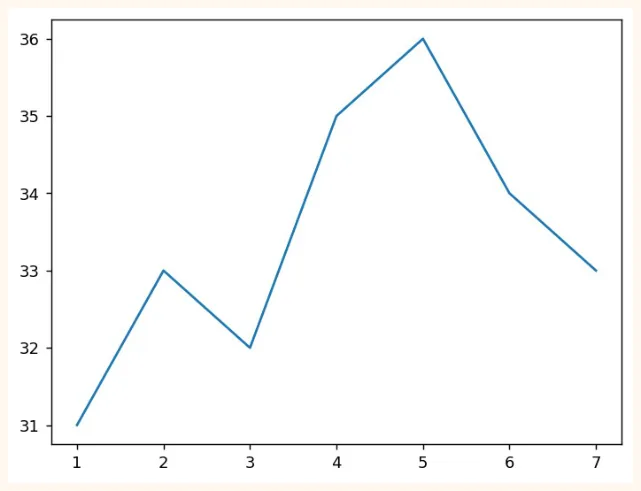
The chart was made in just a few lines. plt.plot(x, y) draws the line, and plt.show() displays it on the screen. But this chart has no title and no labels. A chart like this tells you nothing. Let us fix it.
plt.figure(figsize=(7, 3.8))
plt.plot(days, temp, color="crimson", marker="o", linestyle="--", linewidth=2)
plt.title("Weekly temperature (Karachi)")
plt.xlabel("Day")
plt.ylabel("Temperature (C)")
plt.grid(True, alpha=0.3)
plt.show()
OUTPUT (chart)
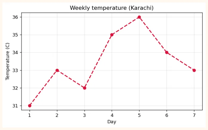
7.3 Two ways of using Matplotlib
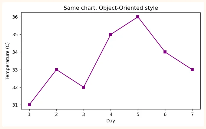
There are two styles of making a chart in Matplotlib. Both are correct, but as charts get bigger the second way is better.
| 1) pyplot style | 2) Object-Oriented (fig, ax) style | |
|---|---|---|
| How | plt.plot(), plt.title()... | fig, ax = plt.subplots(); ax.plot(), ax.set_title() |
| 1) pyplot style | 2) Object-Oriented (fig, ax) style | |
|---|---|---|
| Best when | Small and quick charts | Many charts (subplots), big figures, professional work |
| In short | For small jobs | For more control |
OUTPUT (chart)
7.4 Types of charts (which chart when)
| Chart | When to use | Example question |
|---|---|---|
| Line | Change over time (trend) | How were sales month by month? |
| Bar | Comparison of different categories | How many students are in each city? |
| Histogram | Distributionof one numeric variable | Between which numbers do most students' marks lie? |
| Scatter | Relationship betweentwo numericvariables | Do marks go up as study hours go up? |
| Pie | Share of a whole (few categories, at most 5) | How much of the spending went on what? |
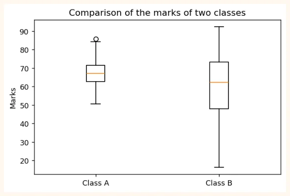
| Box plot | Distribution, median and outliers | Which class has more variation in marks? |
Bar chart
cities = ["Karachi", "Lahore", "Islamabad", "Quetta"]
students = [120, 95, 60, 35]
plt.figure(figsize=(7, 3.8))
plt.bar(cities, students, color=["#A4457A", "#6B5B95", "#E8A5C0", "#2F7D4F"])
plt.title("Students by city")
plt.ylabel("Number of students")
plt.show()
OUTPUT (chart)
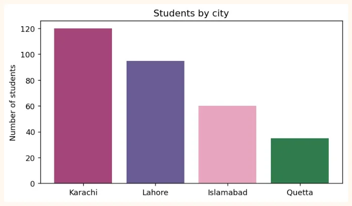
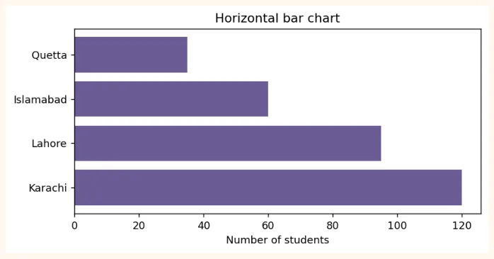
If the names are long, plt.barh() (horizontal bar) works better.
plt.figure(figsize=(7, 3.2))
plt.barh(cities, students, color="#6B5B95")
plt.title("Horizontal bar chart")
plt.xlabel("Number of students")
plt.show()
OUTPUT (chart)
Histogram (looking at a distribution)
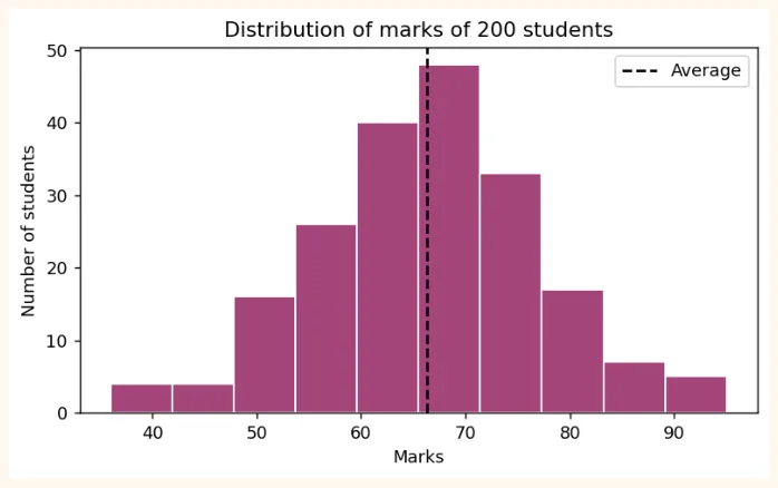
A histogram divides the data into bins (boxes) and shows how many values fell into each bin.
import numpy as np
np.random.seed(1)
marks = np.random.normal(loc=65, scale=12, size=200).round()   # marks of 200 students
plt.figure(figsize=(7, 3.8))
plt.hist(marks, bins=10, color="#A4457A", edgecolor="white")
plt.title("Distribution of marks of 200 students")
plt.xlabel("Marks")
plt.ylabel("Number of students")
plt.axvline(marks.mean(), color="black", linestyle="--", label="Average")
plt.legend()
plt.show()
OUTPUT (chart)
Scatter plot (relationship between two things)
np.random.seed(2)
hours = np.random.uniform(1, 10, 60)                    # study hours
score = 35 + 6 * hours + np.random.normal(0, 6, 60)     # marks (with a little noise)
plt.figure(figsize=(7, 3.8))
plt.scatter(hours, score, color="#6B5B95", alpha=0.7)
plt.title("Study hours and marks")
plt.xlabel("Hours")
plt.ylabel("Marks")
plt.show()
OUTPUT (chart)
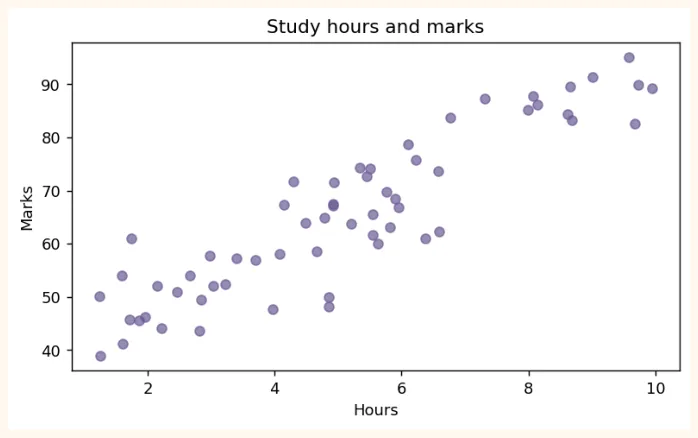
The dots appear to go from the bottom to the top: the more hours, the more marks . This is called positive correlation (in detail in Module 3).
Pie chart
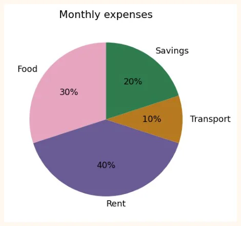
labels = ["Food", "Rent", "Transport", "Savings"]
amounts = [30, 40, 10, 20]
plt.figure(figsize=(5, 4))
plt.pie(amounts, labels=labels, autopct="%1.0f%%", startangle=90,
        colors=["#E8A5C0", "#6B5B95", "#B7791F", "#2F7D4F"])
plt.title("Monthly expenses")
plt.show()
OUTPUT (chart)
Box plot
np.random.seed(3)
class_a = np.random.normal(70, 8, 50)
class_b = np.random.normal(60, 15, 50)
plt.figure(figsize=(6, 3.8))
plt.boxplot([class_a, class_b], tick_labels=["Class A", "Class B"])
plt.title("Comparison of the marks of two classes")
plt.ylabel("Marks")
plt.show()
OUTPUT (chart)
7.5 Plot Customization
| Item | How | Example |
|---|---|---|
| Title / Labels | title(), xlabel(), ylabel() | plt.title("Sales") |
| Colour | color= | "red", "#A4457A" |
| Line style | linestyle= ('-', '--', ':', '-.') | linestyle="--" |
| Line thickness | linewidth= | linewidth=2 |
| Marker | marker= ('o', 's', '^', '*') | marker="o" |
| Transparency | alpha= (0 to 1) | alpha=0.5 |
| Label and Legend | label=, plt.legend() | plt.plot(x, y, label="A") |
| Grid | plt.grid() | plt.grid(True, alpha=0.3) |
| Axis limits | xlim(), ylim() | plt.ylim(0, 100) |
| Axis ticks | xticks(rotation=) | plt.xticks(rotation=45) |
| Chart size | figure(figsize=(w, h)) | figsize=(8, 4) |
| Text / Annotation | annotate(), text() | plt.annotate(...) |
| Style | plt.style.use() | plt.style.use("ggplot") |
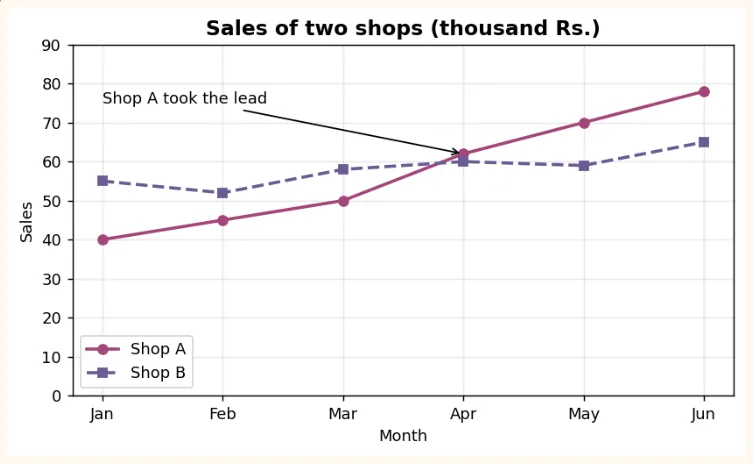
months = ["Jan", "Feb", "Mar", "Apr", "May", "Jun"]
shop_a = [40, 45, 50, 62, 70, 78]
shop_b = [55, 52, 58, 60, 59, 65]
plt.figure(figsize=(7.5, 4))
plt.plot(months, shop_a, marker="o", linewidth=2, color="#A4457A", label="Shop A")
plt.plot(months, shop_b, marker="s", linewidth=2, linestyle="--", color="#6B5B95",
label="Shop B")
plt.title("Sales of two shops (thousand Rs.)", fontsize=13, fontweight="bold")
plt.xlabel("Month")
plt.ylabel("Sales")
plt.ylim(0, 90)
plt.grid(True, alpha=0.3)
plt.legend()
plt.annotate("Shop A took the lead", xy=("Apr", 62), xytext=("Jan", 75),
             arrowprops=dict(arrowstyle="->"))
plt.show()
OUTPUT (chart)
7.6 Subplots (many charts in one figure)
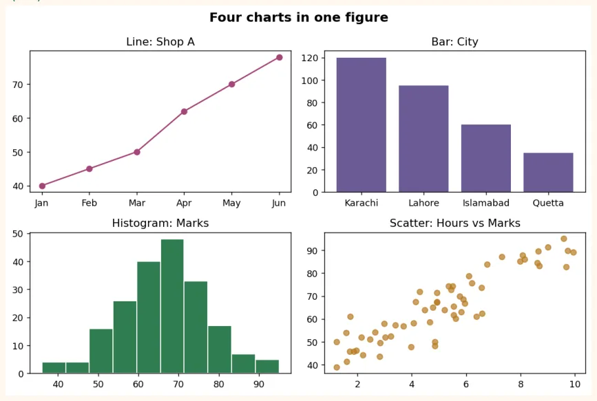
plt.subplots(rows, columns) creates several charts in one figure at once. This is the basic way to build a dashboard.
fig, axes = plt.subplots(2, 2, figsize=(9, 6))
axes[0, 0].plot(months, shop_a, color="#A4457A", marker="o")
axes[0, 0].set_title("Line: Shop A")
axes[0, 1].bar(cities, students, color="#6B5B95")
axes[0, 1].set_title("Bar: City")
axes[1, 0].hist(marks, bins=10, color="#2F7D4F", edgecolor="white")
axes[1, 0].set_title("Histogram: Marks")
axes[1, 1].scatter(hours, score, color="#B7791F", alpha=0.7)
axes[1, 1].set_title("Scatter: Hours vs Marks")
fig.suptitle("Four charts in one figure", fontsize=14, fontweight="bold")
plt.tight_layout()
plt.show()
OUTPUT (chart)
Saving a chart
fig.savefig("dashboard.png", dpi=150, bbox_inches="tight")   # PNG file created
import os
print(os.path.exists("dashboard.png"))
OUTPUT
True
In Colab you can download this file using the folder icon on the left side. The higher the dpi , the sharper the picture.
7.7 Real-world Data Visualization
Now let us put everything together in a real example. We have data for 12 months of sales of a shop. We will build the data with Pandas and answer several questions with charts.
import pandas as pd
import numpy as np
np.random.seed(7)
months = pd.date_range("2025-01-01", periods=12, freq="MS").strftime("%b")
df = pd.DataFrame({
    "month": months,
    "sales": (np.linspace(200, 330, 12) + np.random.normal(0, 15, 12)).round(),
    "ads_budget": np.linspace(20, 60, 12).round() + np.random.randint(-4, 5, 12),
})
df["profit"] = (df["sales"] * 0.25 - df["ads_budget"]).round(1)
print(df.head())
OUTPUT
  month  sales  ads_budget  profit
0   Jan  225.0        22.0    34.2
1   Feb  205.0        23.0    28.2
2   Mar  224.0        28.0    28.0
3   Apr  242.0        35.0    25.5
4   May  235.0        39.0    19.8
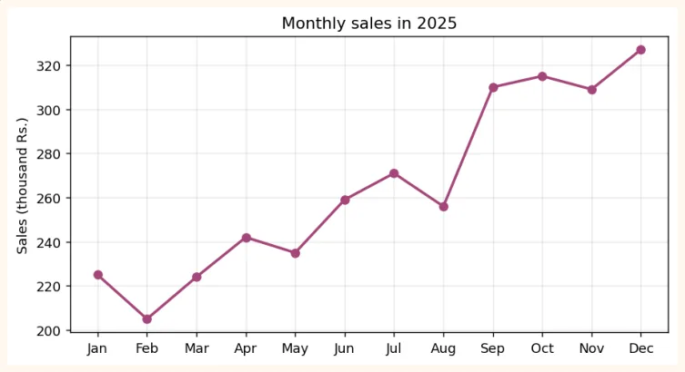
Question 1: What is the trend of sales? (Line chart)
plt.figure(figsize=(8, 4))
plt.plot(df["month"], df["sales"], marker="o", color="#A4457A", linewidth=2)
plt.title("Monthly sales in 2025")
plt.ylabel("Sales (thousand Rs.)")
plt.grid(True, alpha=0.3)
plt.show()
OUTPUT (chart)
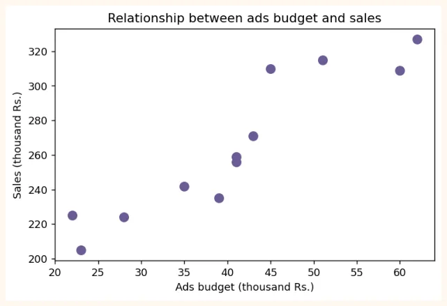
Question 2: Does spending more on ads increase sales? (Scatter)
plt.figure(figsize=(6.5, 4))
plt.scatter(df["ads_budget"], df["sales"], color="#6B5B95", s=70)
plt.title("Relationship between ads budget and sales")
plt.xlabel("Ads budget (thousand Rs.)")
plt.ylabel("Sales (thousand Rs.)")
plt.show()
OUTPUT (chart)
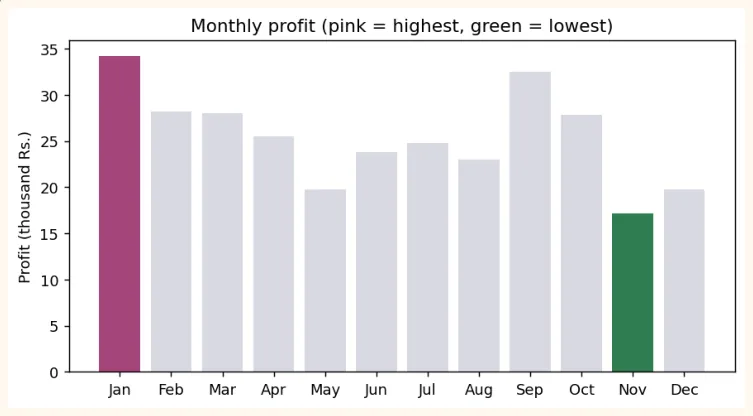
Question 3: In which month was the profit highest and lowest? (Bar)
best = df["profit"].idxmax()
worst = df["profit"].idxmin()
colors = ["#A4457A" if i == best else "#2F7D4F" if i == worst else "#D9D9E3" for i in
df.index]
plt.figure(figsize=(8, 4))
plt.bar(df["month"], df["profit"], color=colors)
plt.title("Monthly profit (pink = highest, green = lowest)")
plt.ylabel("Profit (thousand Rs.)")
plt.show()
print("Highest profit:", df.loc[best, "month"], "|", "Lowest:", df.loc[worst, "month"])
OUTPUT (chart)
GOOD PRACTICE
In real work, do not keep all the bars in one colour. Give a highlight colour to the thing you want to show (highest/lowest) and keep the rest light (grey). This way the viewer understands immediately.
Plotting directly with Pandas
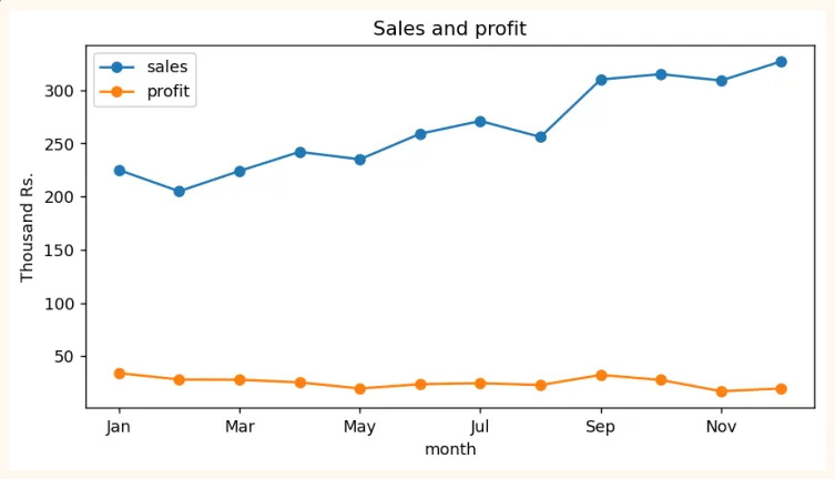
Writing .plot() on a Pandas DataFrame makes a Matplotlib chart directly, with less code.
df.plot(x="month", y=["sales", "profit"], kind="line", marker="o", figsize=(8, 4),
        title="Sales and profit")
plt.ylabel("Thousand Rs.")
plt.show()
OUTPUT (chart)
6 principles of a good chart
-
The title says what the chart shows, and the axis labels carry units (Rs., kg, %).
-
Choose the right chart (line for trend, bar for comparison, scatter for relationship).
-
Always start the y-axis of a bar chart at 0. Otherwise even a small difference looks very big (see below).
-
Use few colours and use them with meaning (highlight). Do not keep more than 5 slices in a pie chart.
-
One point per chart. If you put in too many things, nothing will be understood.
-
Ask the chart yourself: "if I knew nothing about this, would I understand it?"
values = [96, 100]
names = ["Product A", "Product B"]
fig, axes = plt.subplots(1, 2, figsize=(8, 3.4))
axes[0].bar(names, values, color="#6B5B95")
axes[0].set_ylim(94, 101)
axes[0].set_title("Misleading: y-axis starts at 94")
axes[1].bar(names, values, color="#2F7D4F")
axes[1].set_ylim(0, 110)
axes[1].set_title("Correct: y-axis starts at 0")
plt.tight_layout()
plt.show()
OUTPUT (chart)
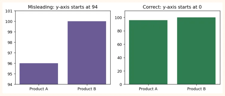
Both charts have the same data (96 and 100). In the first chart B looks several times bigger than A, whereas the difference is only 4%. Charts like this mislead people.
7.8 Hands-on with Matplotlib
Do these exercises on the df of 7.7 (12 months of sales).
-
Line chart: make the trend of ads_budget, with a title and labels.
-
Histogram: make the distribution of sales (bins=6).
-
Bar chart: make a bar chart of the profit of each month, with the months whose profit is below 30 in red.
-
Dual chart: draw the lines of both sales and ads_budget in one chart (with a legend).
-
Subplots: make a line, a bar and a scatter side by side in 1 row and 3 columns, and save it with savefig .
First make them yourself, then compare by changing the code of 7.7. Writing a conclusion in two sentences after looking at the charts is also compulsory practice (for example: "Sales have grown as ads have increased").
KEY TAKEAWAYS
-
A chart tells the story at a glance. A Data Scientist must be able to explain things with charts.
-
Two ways of using Matplotlib: pyplot (plt.plot) and Object-Oriented (fig, ax = plt.subplots()).
-
Line = trend, Bar = comparison, Histogram = distribution, Scatter = relationship between two things, Box = spread and outliers.
-
Customization: title, xlabel, ylabel, color, marker, linestyle, alpha, legend, grid, figsize.
-
Subplots put many charts in one figure, tight_layout() prevents collisions, savefig() saves.
-
Start a bar chart's y-axis at 0, use colour with meaning, and explain your point with a highlight.
-
df.plot() makes a Matplotlib chart directly from Pandas.