Chapter 7: Matplotlib Visualization
MODULE 2 | WEEK 7
Chapter 7: Matplotlib Visualization
Numbers ki lambi tables ko dekh kar kuch samajh nahi aata, lekin ek chart ek nazar me kahani suna deta hai. Data Visualization ka matlab hai data ko tasveer ki shakal dena taake patterns, trends aur ajeeb cheezein foran nazar aa jayen. Matplotlib Python ki sab se bunyadi plotting library hai, aur Seaborn aur Pandas ke charts bhi isi par bane hain.
7.1 Data Visualization kyun?
7.2 Pehla chart: plt.plot()
import matplotlib.pyplot as plt
days = [1, 2, 3, 4, 5, 6, 7]
temp = [31, 33, 32, 35, 36, 34, 33]
plt.plot(days, temp)
plt.show()
OUTPUT (chart)
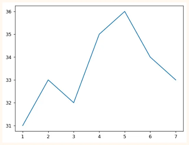
Bas 3 lines me chart ban gaya. plt.plot(x, y) line draw karta hai, aur plt.show() use screen par dikhata hai. Lekin is chart me na title hai, na labels. Aise chart se kuch samajh nahi aata. Isay theek karte hain.
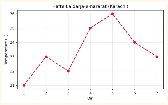
plt.figure(figsize=(7, 3.8))
plt.plot(days, temp, color="crimson", marker="o", linestyle="--", linewidth=2)
plt.title("Hafte ka darja-e-hararat (Karachi)")
plt.xlabel("Din")
plt.ylabel("Temperature (C)")
plt.grid(True, alpha=0.3)
plt.show()
OUTPUT (chart)
7.3 Matplotlib ke do tareeqay
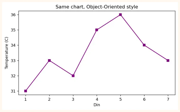
Matplotlib me chart banane ke do style hain. Dono sahi hain, magar jaise jaise charts bare hote hain doosra tareeqa behtar hai.
| 1) pyplot style | 2) Object-Oriented (fig, ax) style | |
|---|---|---|
| Kaise | plt.plot(), plt.title()... | fig, ax = plt.subplots(); ax.plot(), ax.set_title() |
| Kab achha | Chhote aur tez charts | Kai charts (subplots), bari figures, professional kaam |
| 1) pyplot style | 2) Object-Oriented (fig, ax) style | |
|---|---|---|
| Naam | Chhote kaam ke liye | Zyada control ke liye |
OUTPUT (chart)
7.4 Charts ki qismein (kaunsa chart kab)
| Chart | Kab use karein | Misaal sawal |
|---|---|---|
| Line | Waqt ke saath tabdeeli (trend) | Mahine ba mahine sales kaise rahi? |
| Bar | Alag alag categories ka muqabla | Kis shehar me kitne students hain? |
| Histogram | Ek numeric cheez kitaqseem (distribution) | Students ke marks zyada tar kin numbers ke beech hain? |
| Scatter | Do numericcheezon ka rishta | Parhne ke ghantay barhne se marks barhte hain? |
| Pie | Hissa ba hissa (kam categories, 5 se kam) | Kharch ka kitna hissa kis cheez par gaya? |
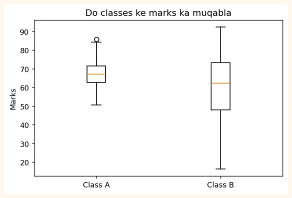
| Box plot | Distribution, median aur outliers | Kis class ke marks me zyada farq hai? |
Bar chart
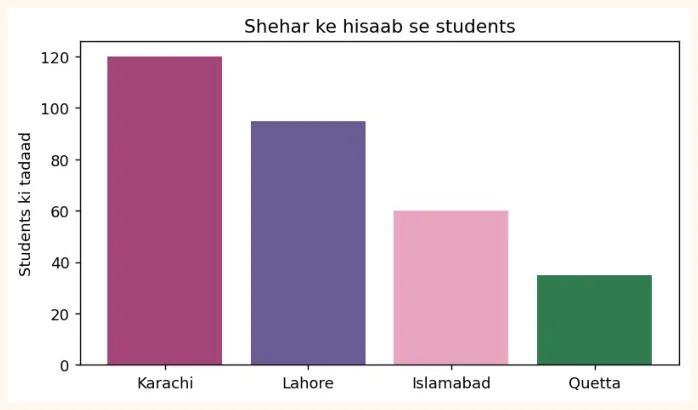
cities = ["Karachi", "Lahore", "Islamabad", "Quetta"]
students = [120, 95, 60, 35]
plt.figure(figsize=(7, 3.8))
plt.bar(cities, students, color=["#A4457A", "#6B5B95", "#E8A5C0", "#2F7D4F"])
plt.title("Shehar ke hisaab se students")
plt.ylabel("Students ki tadaad")
plt.show()
OUTPUT (chart)
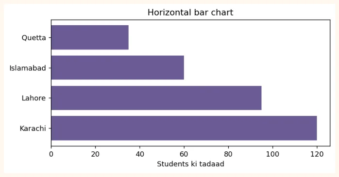
Naam lambay hon to plt.barh() (horizontal bar) behtar rehta hai.
plt.figure(figsize=(7, 3.2))
plt.barh(cities, students, color="#6B5B95")
plt.title("Horizontal bar chart")
plt.xlabel("Students ki tadaad")
plt.show()
OUTPUT (chart)
Histogram (distribution dekhna)
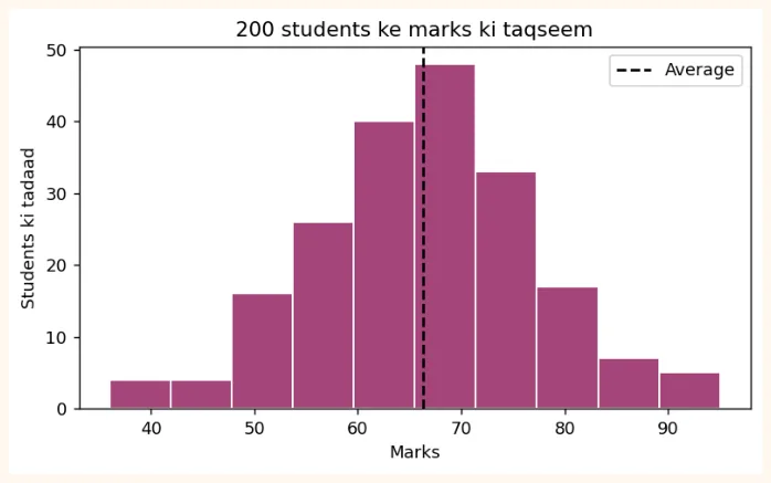
Histogram data ko bins (dibbon) me bant kar dikhata hai ke kis dibbe me kitni values aayin.
import numpy as np
np.random.seed(1)
marks = np.random.normal(loc=65, scale=12, size=200).round()   # 200 students ke marks
plt.figure(figsize=(7, 3.8))
plt.hist(marks, bins=10, color="#A4457A", edgecolor="white")
plt.title("200 students ke marks ki taqseem")
plt.xlabel("Marks")
plt.ylabel("Students ki tadaad")
plt.axvline(marks.mean(), color="black", linestyle="--", label="Average")
plt.legend()
plt.show()
OUTPUT (chart)
Scatter plot (do cheezon ka rishta)
np.random.seed(2)
hours = np.random.uniform(1, 10, 60)                    # parhne ke ghantay
score = 35 + 6 * hours + np.random.normal(0, 6, 60)     # marks (thora shor ke saath)
plt.figure(figsize=(7, 3.8))
plt.scatter(hours, score, color="#6B5B95", alpha=0.7)
plt.title("Parhne ke ghantay aur marks")
plt.xlabel("Ghantay")
plt.ylabel("Marks")
plt.show()
OUTPUT (chart)
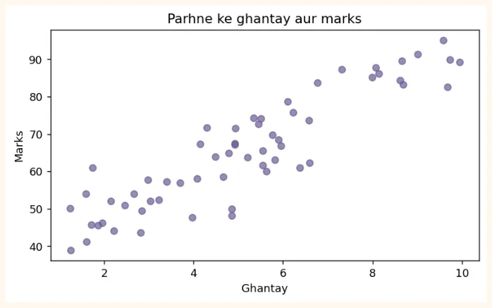
Nuqtay neeche se upar ki taraf jate nazar aa rahe hain: jitne zyada ghantay, utne zyada marks . Isay positive correlation kehte hain (Module 3 me tafseel se).
Pie chart
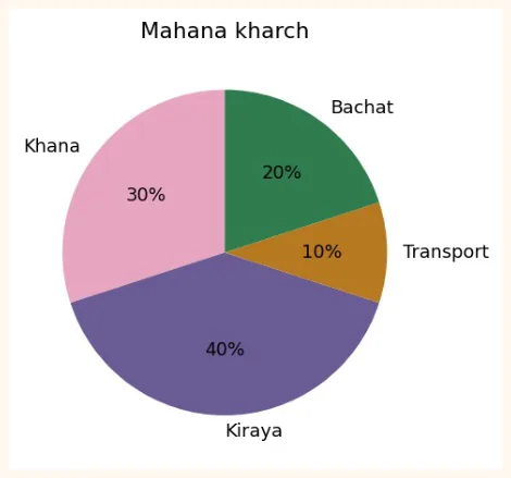
labels = ["Khana", "Kiraya", "Transport", "Bachat"]
amounts = [30, 40, 10, 20]
plt.figure(figsize=(5, 4))
plt.pie(amounts, labels=labels, autopct="%1.0f%%", startangle=90,
        colors=["#E8A5C0", "#6B5B95", "#B7791F", "#2F7D4F"])
plt.title("Mahana kharch")
plt.show()
OUTPUT (chart)
Box plot
np.random.seed(3)
class_a = np.random.normal(70, 8, 50)
class_b = np.random.normal(60, 15, 50)
plt.figure(figsize=(6, 3.8))
plt.boxplot([class_a, class_b], tick_labels=["Class A", "Class B"])
plt.title("Do classes ke marks ka muqabla")
plt.ylabel("Marks")
plt.show()
OUTPUT (chart)
7.5 Plot Customization
| Cheez | Kaise | Misaal |
|---|---|---|
| Title / Labels | title(), xlabel(), ylabel() | plt.title("Sales") |
| Rang | color= | "red", "#A4457A" |
| Line ki shakal | linestyle= ('-', '--', ':', '-.') | linestyle="--" |
| Line ki motai | linewidth= | linewidth=2 |
| Nishan (marker) | marker= ('o', 's', '^', '*') | marker="o" |
| Transparency | alpha= (0 se 1) | alpha=0.5 |
| Label aur Legend | label=, plt.legend() | plt.plot(x, y, label="A") |
| Grid | plt.grid() | plt.grid(True, alpha=0.3) |
| Axis ki hadd | xlim(), ylim() | plt.ylim(0, 100) |
| Axis ke nishan | xticks(rotation=) | plt.xticks(rotation=45) |
| Chart ka size | figure(figsize=(w, h)) | figsize=(8, 4) |
| Text / Annotation | annotate(), text() | plt.annotate(...) |
| Style | plt.style.use() | plt.style.use("ggplot") |
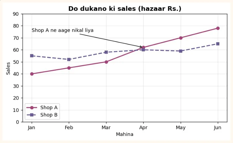
months = ["Jan", "Feb", "Mar", "Apr", "May", "Jun"]
shop_a = [40, 45, 50, 62, 70, 78]
shop_b = [55, 52, 58, 60, 59, 65]
plt.figure(figsize=(7.5, 4))
plt.plot(months, shop_a, marker="o", linewidth=2, color="#A4457A", label="Shop A")
plt.plot(months, shop_b, marker="s", linewidth=2, linestyle="--", color="#6B5B95",
label="Shop B")
plt.title("Do dukano ki sales (hazaar Rs.)", fontsize=13, fontweight="bold")
plt.xlabel("Mahina")
plt.ylabel("Sales")
plt.ylim(0, 90)
plt.grid(True, alpha=0.3)
plt.legend()
plt.annotate("Shop A ne aage nikal liya", xy=("Apr", 62), xytext=("Jan", 75),
             arrowprops=dict(arrowstyle="->"))
plt.show()
OUTPUT (chart)
7.6 Subplots (ek figure me kai charts)
plt.subplots(rows, columns) ek figure me kai charts ek sath banata hai. Ye ek dashboard banane ka bunyadi tareeqa hai.
fig, axes = plt.subplots(2, 2, figsize=(9, 6))
axes[0, 0].plot(months, shop_a, color="#A4457A", marker="o")
axes[0, 0].set_title("Line: Shop A")
axes[0, 1].bar(cities, students, color="#6B5B95")
axes[0, 1].set_title("Bar: Shehar")
axes[1, 0].hist(marks, bins=10, color="#2F7D4F", edgecolor="white")
axes[1, 0].set_title("Histogram: Marks")
axes[1, 1].scatter(hours, score, color="#B7791F", alpha=0.7)
axes[1, 1].set_title("Scatter: Ghantay vs Marks")
fig.suptitle("Chaar charts ek figure me", fontsize=14, fontweight="bold")
plt.tight_layout()
plt.show()
OUTPUT (chart)
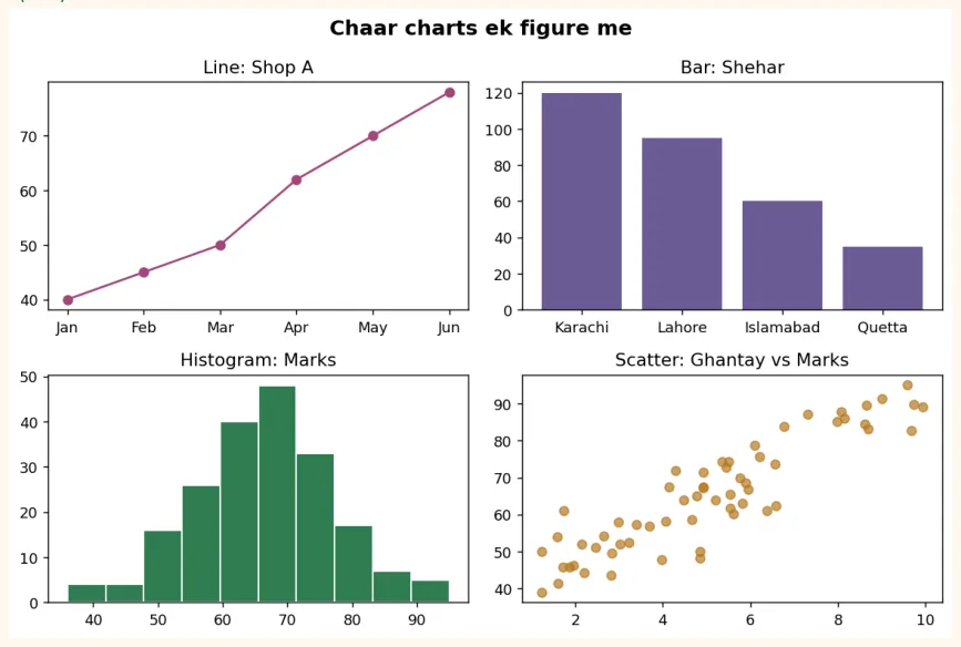
Chart ko save karna
fig.savefig("dashboard.png", dpi=150, bbox_inches="tight")   # PNG file ban gayi
import os
print(os.path.exists("dashboard.png"))
OUTPUT
True
Colab me left side ke folder icon se is file ko download kar sakte ho. dpi jitna zyada, tasveer utni saaf.
7.7 Real-world Data Visualization
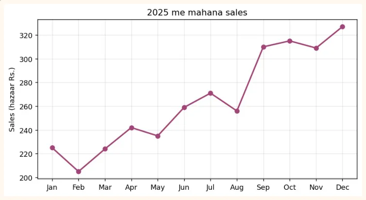
Ab sab kuch ek asli misaal me jorte hain. Hamare paas ek dukaan ki 12 mahine ki sales ka data hai. Hum Pandas se data banayenge, aur kai sawalon ke jawab charts se denge.
import pandas as pd
import numpy as np
np.random.seed(7)
months = pd.date_range("2025-01-01", periods=12, freq="MS").strftime("%b")
df = pd.DataFrame({
    "month": months,
    "sales": (np.linspace(200, 330, 12) + np.random.normal(0, 15, 12)).round(),
    "ads_budget": np.linspace(20, 60, 12).round() + np.random.randint(-4, 5, 12),
})
df["profit"] = (df["sales"] * 0.25 - df["ads_budget"]).round(1)
print(df.head())
OUTPUT
  month  sales  ads_budget  profit
0   Jan  225.0        22.0    34.2
1   Feb  205.0        23.0    28.2
2   Mar  224.0        28.0    28.0
3   Apr  242.0        35.0    25.5
4   May  235.0        39.0    19.8
Sawal 1: Sales ka trend kya hai? (Line chart)
plt.figure(figsize=(8, 4))
plt.plot(df["month"], df["sales"], marker="o", color="#A4457A", linewidth=2)
plt.title("2025 me mahana sales")
plt.ylabel("Sales (hazaar Rs.)")
plt.grid(True, alpha=0.3)
plt.show()
OUTPUT (chart)
Sawal 2: Kya ads par zyada paisa lagane se sales barhti hain? (Scatter)
plt.figure(figsize=(6.5, 4))
plt.scatter(df["ads_budget"], df["sales"], color="#6B5B95", s=70)
plt.title("Ads budget aur sales ka rishta")
plt.xlabel("Ads budget (hazaar Rs.)")
plt.ylabel("Sales (hazaar Rs.)")
plt.show()
OUTPUT (chart)
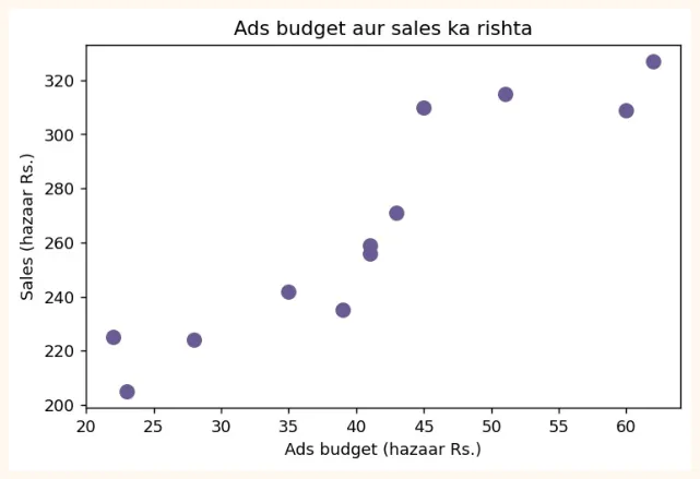
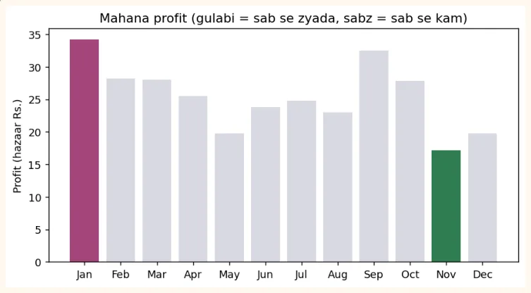
Sawal 3: Kaunse mahine me sab se zyada aur sab se kam profit hua? (Bar)
best = df["profit"].idxmax()
worst = df["profit"].idxmin()
colors = ["#A4457A" if i == best else "#2F7D4F" if i == worst else "#D9D9E3" for i in
df.index]
plt.figure(figsize=(8, 4))
plt.bar(df["month"], df["profit"], color=colors)
plt.title("Mahana profit (gulabi = sab se zyada, sabz = sab se kam)")
plt.ylabel("Profit (hazaar Rs.)")
plt.show()
print("Sab se zyada profit:", df.loc[best, "month"], "|", "Sab se kam:", df.loc[worst,
"month"])
OUTPUT (chart)
ACHHA TAREEQA
Asli kaam me sab charts ek hi rang ke na rakho. Jo baat dikhani hai (sab se zyada/kam) usay highlight rang do aur baqi ko halka (grey) rakho. Is se dekhne wale ko foran samajh aa jata hai.
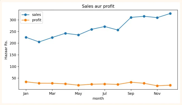
Pandas se seedha plot
Pandas ke DataFrame par .plot() likhne se Matplotlib ka chart seedha ban jata hai, kam code me.
df.plot(x="month", y=["sales", "profit"], kind="line", marker="o", figsize=(8, 4),
        title="Sales aur profit")
plt.ylabel("Hazaar Rs.")
plt.show()
OUTPUT (chart)
Achhe chart ke 6 usool
-
Title batay ke chart kya dikha raha hai, aur axes ke labels me units likho (Rs., kg, %).
-
Sahi chart chuno (trend ke liye line, muqabla ke liye bar, rishta ke liye scatter).
-
Bar chart ka y-axis hamesha 0 se shuru karo. Warna chhota farq bhi bohat bara lagta hai (neeche dekho).
-
Rang kam rakho aur maani ke saath (highlight). Pie chart me 5 se zyada hisse na rakho.
-
Ek chart me ek hi baat. Zyada cheezein dalo gi to kuch samajh nahi aayega.
-
Chart ko apne aap se poocho: "agar mujhe iske baare me kuch nahi pata, kya ye samajh aa raha hai?"
values = [96, 100]
names = ["Product A", "Product B"]
fig, axes = plt.subplots(1, 2, figsize=(8, 3.4))
axes[0].bar(names, values, color="#6B5B95")
axes[0].set_ylim(94, 101)
axes[0].set_title("Gumrah-kun: y-axis 94 se shuru")
axes[1].bar(names, values, color="#2F7D4F")
axes[1].set_ylim(0, 110)
axes[1].set_title("Sahi: y-axis 0 se shuru")
plt.tight_layout()
plt.show()
OUTPUT (chart)
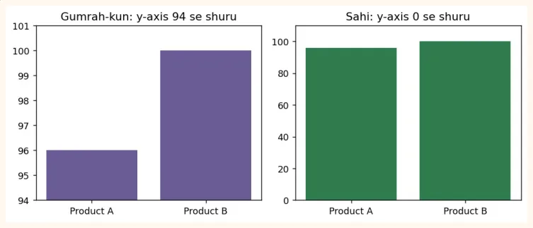
Dono charts me wohi data hai (96 aur 100). Pehle chart me B, A se kai guna bara lagta hai, jab ke farq sirf 4% hai. Is tarah ke chart logon ko gumrah karte hain.
AAM GALTIYAN
-
plt.show() bhool jana (Colab me aksar khud dikh jata hai, lekin script me nahi).
-
Title aur axis labels na likhna.
-
Bar chart ka y-axis 0 se na shuru karna.
-
Pie chart me bohat zyada hisse rakhna.
-
Subplots me tight_layout() na lagana, jis se titles aapas me takra jate hain.
-
Ek hi cell me kai charts banate waqt plt.figure() na likhna, jis se charts ek doosre par ban jate hain.
-
Hamesha line chart use karna. Categories ke liye bar chart behtar hai.
7.8 Hands-on with Matplotlib
Ye exercises 7.7 wale df (12 mahine ki sales) par karo.
-
Line chart: ads_budget ka trend banao, title aur labels ke saath.
-
Histogram: sales ki taqseem (bins=6) banao.
-
Bar chart: har mahine ke profit ka bar chart banao jis me jin mahinon ka profit 30 se kam ho wo laal ho.
-
Dual chart: ek hi chart me sales aur ads_budget dono ki line banao (legend ke saath).
-
Subplots: 1 row aur 3 columns me line, bar aur scatter ek sath banao aur savefig se save karo.
Pehle khud banao, phir 7.7 ke codes me tabdeeli karke compare karo. Charts ko dekh kar do jumlon me nateeja likhna bhi lazmi practice hai (jaise: "Ads barhane ke saath sales barhi hain").
KEY TAKEAWAYS
-
Chart ek nazar me kahani suna deta hai. Data Scientist ko chart se baat samjhana aani chahiye.
-
Matplotlib ke do tareeqay: pyplot (plt.plot) aur Object-Oriented (fig, ax = plt.subplots()).
-
Line = trend, Bar = muqabla, Histogram = distribution, Scatter = do cheezon ka rishta, Box = spread aur outliers.
-
Customization: title, xlabel, ylabel, color, marker, linestyle, alpha, legend, grid, figsize.
-
Subplots se ek figure me kai charts, tight_layout() se takrao se bachao, savefig() se save karo.
-
Bar chart ka y-axis 0 se shuru karo, rang maani ke saath use karo, aur highlight se baat samjhao.
-
df.plot() Pandas se seedha Matplotlib chart banata hai.