Chapter 8: Seaborn and Visualization Project
MODULE 2 | WEEK 8
Chapter 8: Seaborn and Visualization Project
Matplotlib is very powerful, but making a good chart takes quite a lot of code. Seaborn is a library built on top of Matplotlib that makes beautiful statistical charts with less code , and works directly with a Pandas DataFrame. At the end of this chapter we will build a complete Visualization Project .
8.1 What is Seaborn?
OUTPUT
(244, 7) | |
|---|---|
total_bill | tip sex smoker day time size |
0 16.99 | 1.01 Female No Sun Dinner 2 |
1 10.34 | 1.66 Male No Sun Dinner 3 |
2 21.01 | 3.50 Male No Sun Dinner 3 |
3 23.68 | 3.31 Male No Sun Dinner 2 |
4 24.59 | 3.61 Female No Sun Dinner 4 |
The tips dataset contains 244 bills from one restaurant. Columns: total_bill (the bill, in dollars), tip (the tip), sex (gender of the person paying), smoker (whether it was a smoking table or not), day (the day), time (Lunch or Dinner), size (how many people were at the table).
tips.info()
print(tips.describe().round(2))
OUTPUT
<class 'pandas.DataFrame'> |
|---|
RangeIndex: 244 entries, 0 to 243 |
Data columns (total 7 columns): |
# Column Non-Null Count Dtype |
--- ------ -------------- ----- |
0 total_bill 244 non-null float64 |
1 tip 244 non-null float64 |
2 sex 244 non-null category |
3 smoker 244 non-null category |
4 day 244 non-null category |
5 time 244 non-null category |
6 size 244 non-null int64 |
dtypes: category(4), float64(2), int64(1) |
memory usage: 7.4 KB |
total_bill tip size |
count 244.00 244.00 244.00 |
mean 19.79 3.00 2.57 |
std 8.90 1.38 0.95 |
min 3.07 1.00 1.00 |
25% 13.35 2.00 2.00 |
50% 17.80 2.90 2.00 |
75% 24.13 3.56 3.00 |
max 50.81 10.00 6.00 |
8.2 Themes and Color Palettes
sns.set_theme() changes the look of all charts in the whole notebook in one line.
| style= | Look |
|---|---|
| "darkgrid" (default) | Dark background, grid |
| "whitegrid" | White background, grid (common for reports) |
| "white" | Clean white, no grid |
| "ticks" | Tick marks on the axes |
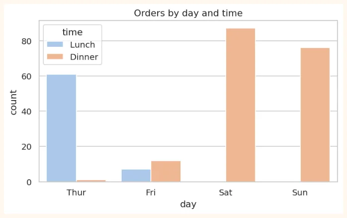
sns.set_theme(style="whitegrid", palette="pastel")
plt.figure(figsize=(7, 3.8))
sns.countplot(data=tips, x="day", hue="time")
plt.title("Orders by day and time")
plt.show()
OUTPUT (chart)
8.3 Distribution Plots (the spread of data)
These show where the values of a numeric column are high or low.
histplot (a better form of the histogram)
fig, axes = plt.subplots(1, 2, figsize=(10, 3.8))
sns.histplot(data=tips, x="total_bill", bins=20, kde=True, ax=axes[0])
axes[0].set_title("Distribution of bill (kde=True: with a curve)")
sns.histplot(data=tips, x="total_bill", hue="time", multiple="stack", ax=axes[1])
axes[1].set_title("Lunch and Dinner in different colours")
plt.tight_layout()
plt.show()
OUTPUT (chart)
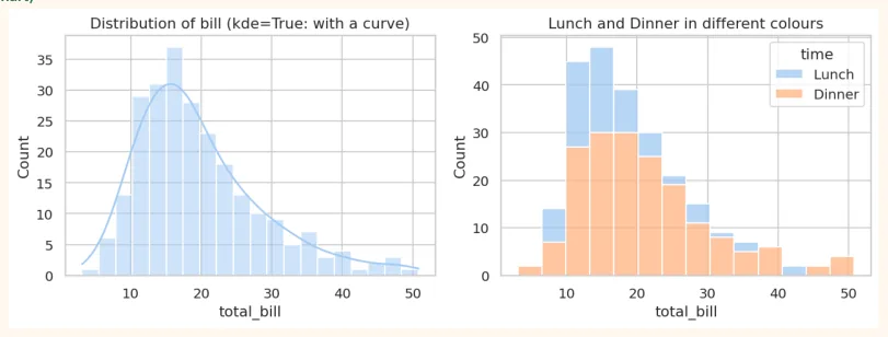
kde (Kernel Density Estimate) is a smooth curve over the histogram that shows the shape of the distribution.
boxplot and violinplot
fig, axes = plt.subplots(1, 2, figsize=(10, 3.8))
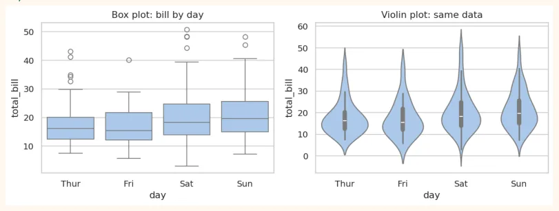
sns.boxplot(data=tips, x="day", y="total_bill", ax=axes[0])
axes[0].set_title("Box plot: bill by day")
sns.violinplot(data=tips, x="day", y="total_bill", ax=axes[1])
axes[1].set_title("Violin plot: same data")
plt.tight_layout()
plt.show()
OUTPUT (chart)
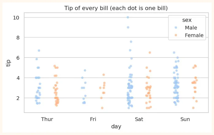
stripplot and swarmplot (every dot separate)
plt.figure(figsize=(7, 3.8))
sns.stripplot(data=tips, x="day", y="tip", hue="sex", dodge=True, alpha=0.7)
plt.title("Tip of every bill (each dot is one bill)")
plt.show()
OUTPUT (chart)
8.4 Categorical Plots
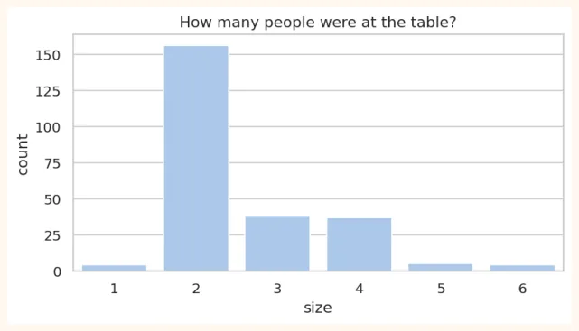
countplot (how many rows in each category)
plt.figure(figsize=(7, 3.4))
sns.countplot(data=tips, x="size")
plt.title("How many people were at the table?")
plt.show()
OUTPUT (chart)
barplot (the average of each category)
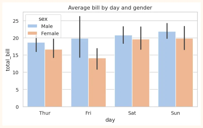
barplot shows the average of each category, and on top of it there is a black line (error bar) that tells you how reliable this average is (confidence interval, in Module 3).
plt.figure(figsize=(7, 3.8))
sns.barplot(data=tips, x="day", y="total_bill", hue="sex")
plt.title("Average bill by day and gender")
plt.show()
OUTPUT (chart)
# barplot does inside what groupby gives
print(tips.groupby("day", observed=True)["total_bill"].mean().round(2))
OUTPUT
day
Thur 17.68
Fri 17.15
Sat 20.44
Sun 21.41
Name: total_bill, dtype: float64
8.5 Relational Plots (the relationship between two things)
scatterplot (with hue, size, style)
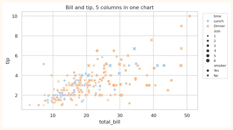
In Seaborn, one scatter plot can show several more columns too: colour ( hue ), dot size ( size ), dot shape ( style ).
plt.figure(figsize=(7.5, 4.2))
sns.scatterplot(data=tips, x="total_bill", y="tip", hue="time", size="size", style="smoker")
plt.title("Bill and tip, 5 columns in one chart")
plt.legend(bbox_to_anchor=(1.02, 1), loc="upper left", fontsize=8)
plt.show()
OUTPUT (chart)
regplot / lmplot (scatter + trend line)
plt.figure(figsize=(7, 4))
sns.regplot(data=tips, x="total_bill", y="tip", line_kws={"color": "red"})
plt.title("How the tip grows as the bill grows")
plt.show()
OUTPUT (chart)
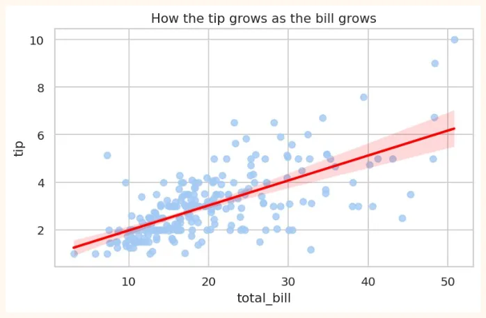
The red line is the regression line : it is the best straight line passing through the middle of the data. It will be explained fully in Module 3 (Week 11).
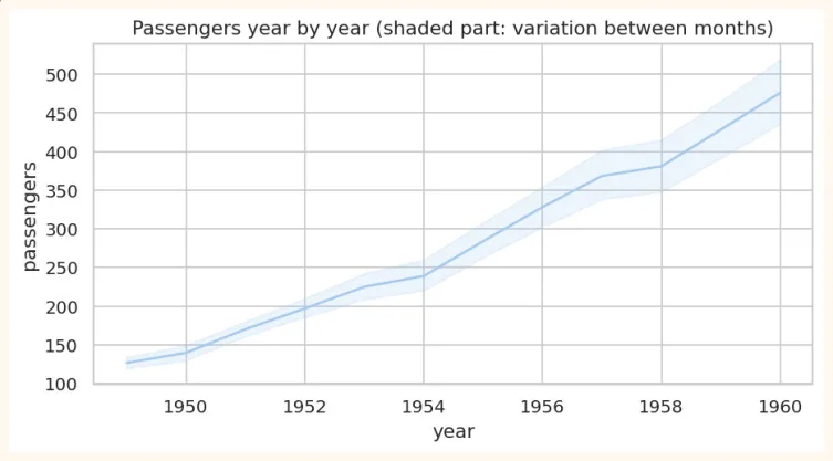
lineplot (trend over time)
flights = sns.load_dataset("flights") # monthly passengers from 1949 to 1960
print(flights.head(3))
OUTPUT
year month passengers
0 1949 Jan 112
1 1949 Feb 118
2 1949 Mar 132
plt.figure(figsize=(8, 3.8))
sns.lineplot(data=flights, x="year", y="passengers")
plt.title("Passengers year by year (shaded part: variation between months)")
plt.show()
OUTPUT (chart)
8.6 Heatmap and Correlation
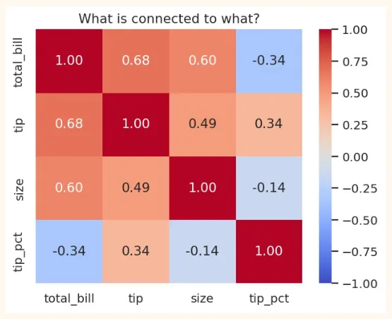
Correlation tells the relationship between two numeric columns as a number between -1 and +1 .
| Correlation | Meaning | Example |
|---|---|---|
| +1 | Perfect direct relationship: when one rises, the other rises too | Study hours and marks (roughly) |
| 0 | No relationship | Shoe size and marks |
| -1 | Perfect opposite relationship: when one rises, the other falls | Speed of a car and travel time |
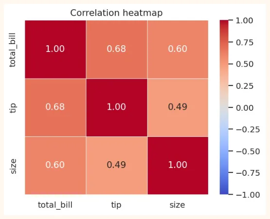
corr = tips[["total_bill", "tip", "size"]].corr()
print(corr.round(2))
OUTPUT
total_bill tip size |
|---|
total_bill 1.00 0.68 0.60 |
tip 0.68 1.00 0.49 |
size 0.60 0.49 1.00 |
Reading numbers is a bit hard. A heatmap shows this table in colours : the darker the colour, the stronger the relationship.
OUTPUT (chart)
-
annot=True: write the number in each box.
-
cmap=: the colour palette (coolwarm, viridis, Blues...).
-
vmin / vmax: the colour limits (-1 and 1 for correlation).
-
fmt=".2f": the number up to 2 decimals.
VERY IMPORTANT
Correlation does not mean causation. In summer, both ice-cream sales and drowning accidents go up, but ice cream does not drown anyone. The cause of both is the heat . Correlation only tells the relationship, not the cause.
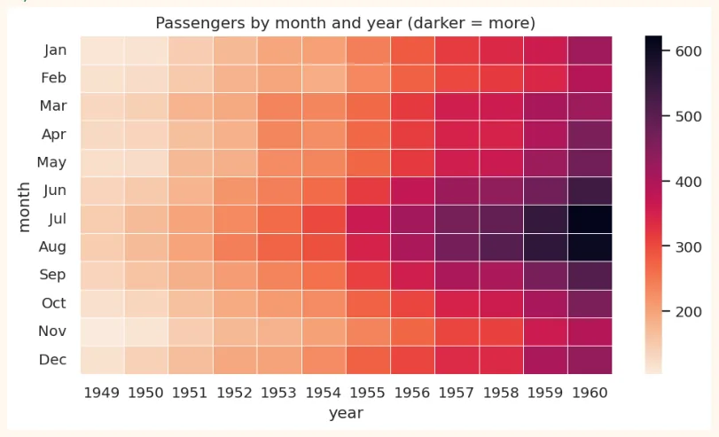
Another use of a heatmap: showing a pivot table
pivot = flights.pivot(index="month", columns="year", values="passengers")
plt.figure(figsize=(9, 4.6))
sns.heatmap(pivot, cmap="rocket_r", linewidths=0.3)
plt.title("Passengers by month and year (darker = more)")
plt.show()
OUTPUT (chart)
8.7 Pairplot, Jointplot and relplot
pairplot (every column against every other)
In one line you get a scatter plot of every numeric column against the others , and on the diagonal a histogram of each column (or a smooth KDE curve when you use hue). It is a very handy tool for taking a first look at new data.
penguins = sns.load_dataset("penguins").dropna() # data of 3 species of penguins
print(penguins.shape)
sns.pairplot(penguins, hue="species", vars=["bill_length_mm", "flipper_length_mm",
"body_mass_g"],
height=2.2)
plt.show()
OUTPUT (chart)
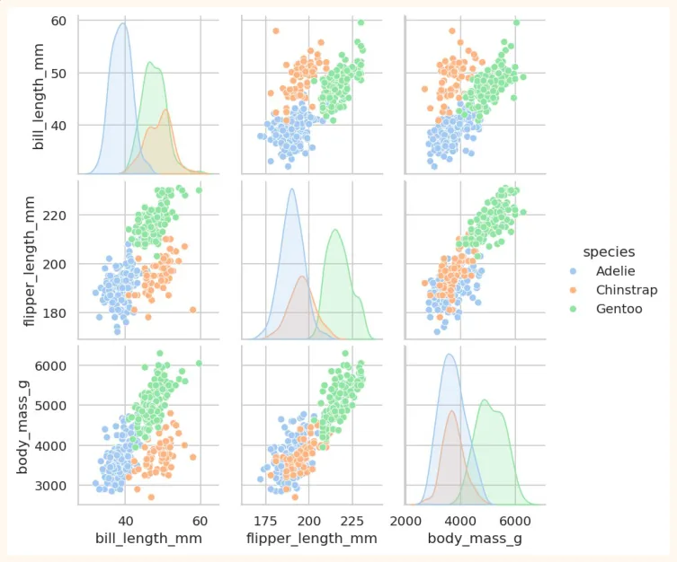
See how the three colours (three species) appear as separate, roundish groups. This is exactly what helps ML in classification : if the groups look separate, a model can separate them easily.
jointplot (the relationship between two things and their own distributions)
sns.jointplot(data=tips, x="total_bill", y="tip", kind="scatter", height=5)
plt.show()
OUTPUT (chart)
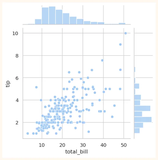
relplot / FacetGrid (a separate chart for each category)
sns.relplot(data=tips, x="total_bill", y="tip", col="time", row="smoker", hue="sex",
height=2.4, aspect=1.4)
plt.show()
OUTPUT (chart)
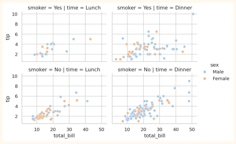
8.8 Customizing and saving Seaborn charts
Seaborn is built on Matplotlib, so everything from Matplotlib (title, labels, figsize, savefig) works here too.
fig, ax = plt.subplots(figsize=(6, 3.6))
sns.boxplot(data=tips, x="time", y="tip", ax=ax, palette="Set2", hue="time", dodge=False,
legend=False)
ax.set_title("Lunch vs Dinner: tip")
ax.set_xlabel("Time")
ax.set_ylabel("Tip (dollars)")
fig.savefig("tips_box.png", dpi=150, bbox_inches="tight")
print("Saved!")
OUTPUT
Saved!
8.9 Visualization Project: Restaurant Tips Analysis
So far we have learned the tools of Matplotlib, Pandas and Seaborn. Now let us combine them all in one real project. The owner of a restaurant asks you: "How do my customers tip, and what does it depend on?"
Aim of the project
-
Load, inspect and clean the data.
-
Create a new column: tip_pct (what percent of the bill was given as tip).
-
Answer at least 4 questions with charts.
-
Finally, write insights and recommendations .
Step 1: Load the data and take a first look
import pandas as pd
import seaborn as sns
import matplotlib.pyplot as plt
tips = sns.load_dataset("tips")
print("Shape:", tips.shape)
print("Missing values:", tips.isnull().sum().sum())
print("Duplicates:", tips.duplicated().sum())
OUTPUT
Shape: (244, 7)
Missing values: 0
Duplicates: 1
There is one duplicate row. This is real data in which two different bills can be exactly the same, so in this project we keep it. In cleaning, always decide after thinking .
Step 2: The new column
tips["tip_pct"] = (tips["tip"] / tips["total_bill"] * 100).round(2)
print(tips["tip_pct"].describe().round(2))
OUTPUT
count 244.00
mean 16.08
std 6.11
min 3.56
25% 12.91
50% 15.48
75% 19.15
max 71.03
Name: tip_pct, dtype: float64
Step 3: Answering the questions (with numbers)
print("Question 1: smokers or non-smokers, whose average tip%?")
print(tips.groupby("smoker", observed=True)["tip_pct"].mean().round(2))
print("\nQuestion 2: which day has the highest tip%?")
print(tips.groupby("day", observed=True)["tip_pct"].mean().round(2))
print("\nQuestion 3: Lunch or Dinner?")
print(tips.groupby("time", observed=True)["tip_pct"].mean().round(2))
print("\nQuestion 4: table size and tip%")
print(tips.groupby("size", observed=True)["tip_pct"].mean().round(2))
OUTPUT
Question 1: smokers or non-smokers, whose average tip%?
smoker
Yes 16.32
No 15.93
Name: tip_pct, dtype: float64
Question 2: which day has the highest tip%?
day
Thur 16.13
Fri 16.99
Sat 15.31
Sun 16.69
Name: tip_pct, dtype: float64
Question 3: Lunch or Dinner?
time
Lunch 16.41
Dinner 15.95
Name: tip_pct, dtype: float64
Question 4: table size and tip%
size
1 21.73
2 16.57
3 15.21
4 14.59
5 14.15
6 15.62
Name: tip_pct, dtype: float64
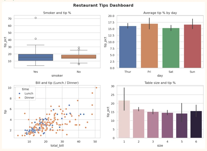
Step 4: Dashboard (4 charts in one figure)
sns.set_theme(style="whitegrid")
fig, axes = plt.subplots(2, 2, figsize=(11, 8))
sns.boxplot(data=tips, x="smoker", y="tip_pct", hue="smoker", dodge=False, legend=False,
ax=axes[0, 0])
axes[0, 0].set_title("Smoker and tip %")
sns.barplot(data=tips, x="day", y="tip_pct", hue="day", dodge=False, legend=False,
ax=axes[0, 1])
axes[0, 1].set_title("Average tip % by day")
sns.scatterplot(data=tips, x="total_bill", y="tip", hue="time", ax=axes[1, 0])
axes[1, 0].set_title("Bill and tip (Lunch / Dinner)")
sns.barplot(data=tips, x="size", y="tip_pct", hue="size", legend=False, ax=axes[1, 1])
axes[1, 1].set_title("Table size and tip %")
fig.suptitle("Restaurant Tips Dashboard", fontsize=15, fontweight="bold")
plt.tight_layout()
plt.show()
OUTPUT (chart)
Step 5: Correlation
plt.figure(figsize=(5.5, 4.2))
sns.heatmap(tips[["total_bill", "tip", "size", "tip_pct"]].corr(), annot=True,
            cmap="coolwarm", vmin=-1, vmax=1, fmt=".2f")
plt.title("What is connected to what?")
plt.show()
OUTPUT (chart)
Step 6: Write the insights yourself
Look at the charts and numbers and write 4 to 5 sentences in your own words . The format, for example:
• Observation: "As the bill grows, the tip amount grows (the correlation is strong)."
-
But: "the tip percent does not grow as much with the bill, which means people give roughly the same percent as tip."
-
Answer to the question: "There is a ___ difference in the tip percent of smokers and non-smokers." (fill it from your output)
-
Recommendation: "The restaurant should focus on ___." (with a reason from the data)
How to put the project on GitHub
-
Create a folder: tips-analysis . Put the notebook ( .ipynb ) in it (from Colab: File > Download > .ipynb).
-
Write a README.md : project name, aim, dataset, tools (Pandas, Seaborn), screenshots of 3 to 4 charts, and the insights.
-
Create a new repository on GitHub and upload the files.
-
Add the link of the repository to your CV or LinkedIn.
8.10 Hands-on with Seaborn
Practise on the Penguins dataset (small data science questions):
import seaborn as sns
import matplotlib.pyplot as plt
penguins = sns.load_dataset("penguins").dropna()
print(penguins.head(3))
print(penguins["species"].value_counts())
OUTPUT
  species     island  bill_length_mm  bill_depth_mm  flipper_length_mm  \
0  Adelie  Torgersen            39.1           18.7              181.0
1  Adelie  Torgersen            39.5           17.4              186.0
2  Adelie  Torgersen            40.3           18.0              195.0
   body_mass_g     sex
0       3750.0    Male
1       3800.0  Female
2       3250.0  Female
species
Adelie       146
Gentoo       119
Chinstrap     68
Name: count, dtype: int64
-
countplot: the number of penguins of each species (with separate colours by island).
-
histplot: the distribution of body_mass_g, with a separate colour for each species ( hue="species" ).
-
boxplot: flipper_length_mm by species. Which species has the longest flippers?
-
scatterplot: bill_length_mm vs bill_depth_mm, coloured by species. Do the three groups look separate? 5. heatmap: the correlation of the numeric columns of penguins. Which two columns have the strongest relationship?
-
pairplot: the whole dataset with hue="sex" . Do male and female penguins look different?
Bonus challenge: find a dataset of your own (a CSV from Kaggle or elsewhere) and make a small visualization project using the methods of this chapter. This will be a good first project for your portfolio.
KEY TAKEAWAYS
-
Seaborn is built on Matplotlib: less code, a beautiful default look, works directly with a DataFrame.
-
sns.set_theme() changes the look of the whole notebook.
-
Distribution: histplot, kdeplot, boxplot, violinplot, stripplot. Categorical: countplot, barplot.
-
Relational: scatterplot (hue, size, style), lineplot, regplot.
-
A heatmap shows correlation (-1 to +1) in colours. Correlation does not mean causation.
-
pairplot is an excellent way to take a first look at new data. relplot/FacetGrid gives a separate chart for each category.
-
Real insights are those that tell you what it means and what to do now.