Chapter 8: Seaborn aur Visualization Project
MODULE 2 | WEEK 8
Chapter 8: Seaborn aur Visualization Project
Matplotlib bohat taqatwar hai magar ek achha chart banane ke liye kafi code likhna parta hai. Seaborn Matplotlib ke upar bani hui library hai jo kam code me khoobsurat aur statistical charts banati hai, aur seedha Pandas DataFrame ke saath kaam karti hai. Is chapter ke aakhir me hum ek poora Visualization Project banayenge.
8.1 Seaborn kya hai?
OUTPUT
(244, 7)
total_bill tip sex smoker day time size
0 16.99 1.01 Female No Sun Dinner 2
1 10.34 1.66 Male No Sun Dinner 3
2 21.01 3.50 Male No Sun Dinner 3
3 23.68 3.31 Male No Sun Dinner 2
4 24.59 3.61 Female No Sun Dinner 4
tips dataset me ek restaurant ke 244 bills hain. Columns: total_bill (bill, dollars), tip (tip), sex (bill dene wale ki jins), smoker (smoker table tha ya nahi), day (din), time (Lunch ya Dinner), size (table par kitne log the).
tips.info()
print(tips.describe().round(2))
OUTPUT
<class 'pandas.DataFrame'>
RangeIndex: 244 entries, 0 to 243
Data columns (total 7 columns):
# Column Non-Null Count Dtype
--- ------ -------------- -----
0 total_bill 244 non-null float64
1 tip 244 non-null float64
2 sex 244 non-null category
3 smoker 244 non-null category
4 day 244 non-null category
5 time 244 non-null category
6 size 244 non-null int64
dtypes: category(4), float64(2), int64(1)
memory usage: 7.4 KB
total_bill tip size
count 244.00 244.00 244.00
mean 19.79 3.00 2.57
std 8.90 1.38 0.95
min 3.07 1.00 1.00
25% 13.35 2.00 2.00
50% 17.80 2.90 2.00
75% 24.13 3.56 3.00
max 50.81 10.00 6.00
8.2 Themes aur Color Palettes
sns.set_theme() ek line me poore notebook ke charts ka look badal deta hai.
| style= | Look |
|---|---|
| "darkgrid" (default) | Dark background, grid |
| "whitegrid" | Safed background, grid (report ke liye aam) |
| "white" | Saaf safed, koi grid nahi |
| "ticks" | Axes par nishan |
sns.set_theme(style="whitegrid", palette="pastel")
plt.figure(figsize=(7, 3.8))
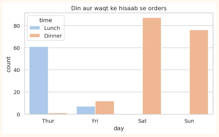
sns.countplot(data=tips, x="day", hue="time")
plt.title("Din aur waqt ke hisaab se orders")
plt.show()
OUTPUT (chart)
8.3 Distribution Plots (data ki taqseem)
Ye batate hain ke ek numeric column ki values kahan kahan zyada ya kam hain.
histplot (histogram ka behtar roop)
fig, axes = plt.subplots(1, 2, figsize=(10, 3.8))
sns.histplot(data=tips, x="total_bill", bins=20, kde=True, ax=axes[0])
axes[0].set_title("Bill ki taqseem (kde=True: lakeer ke saath)")
sns.histplot(data=tips, x="total_bill", hue="time", multiple="stack", ax=axes[1])
axes[1].set_title("Lunch aur Dinner alag rang me")
plt.tight_layout()
plt.show()
OUTPUT (chart)
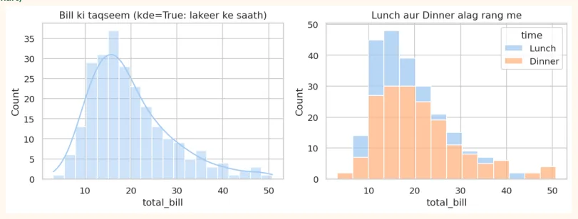
kde (Kernel Density Estimate) histogram ke upar ek smooth lakeer hai jo taqseem ki shakal dikhati hai.
boxplot aur violinplot
fig, axes = plt.subplots(1, 2, figsize=(10, 3.8))
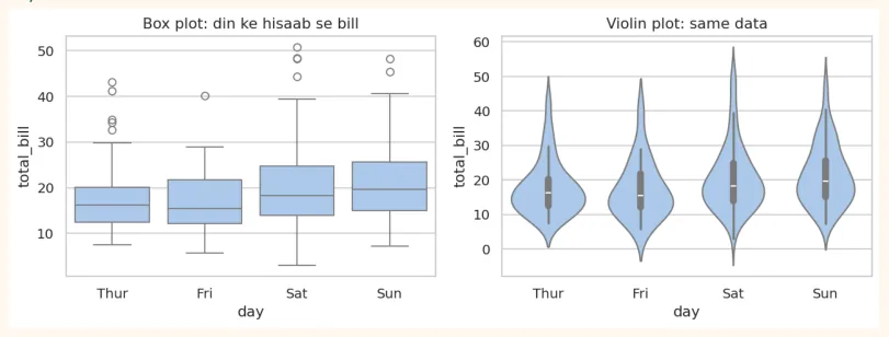
sns.boxplot(data=tips, x="day", y="total_bill", ax=axes[0])
axes[0].set_title("Box plot: din ke hisaab se bill")
sns.violinplot(data=tips, x="day", y="total_bill", ax=axes[1])
axes[1].set_title("Violin plot: same data")
plt.tight_layout()
plt.show()
OUTPUT (chart)
stripplot aur swarmplot (har nuqta alag)
plt.figure(figsize=(7, 3.8))
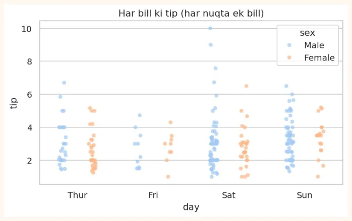
sns.stripplot(data=tips, x="day", y="tip", hue="sex", dodge=True, alpha=0.7)
plt.title("Har bill ki tip (har nuqta ek bill)")
plt.show()
OUTPUT (chart)
8.4 Categorical Plots
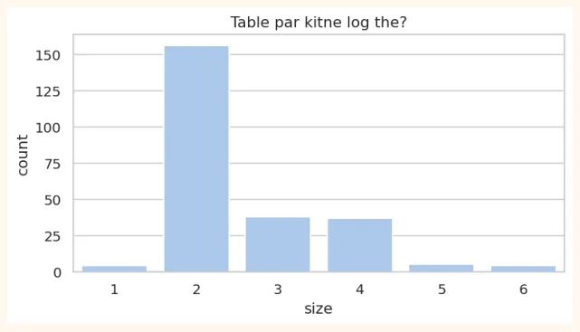
countplot (har category me kitni rows)
plt.figure(figsize=(7, 3.4))
sns.countplot(data=tips, x="size")
plt.title("Table par kitne log the?")
plt.show()
OUTPUT (chart)
barplot (har category ka average)
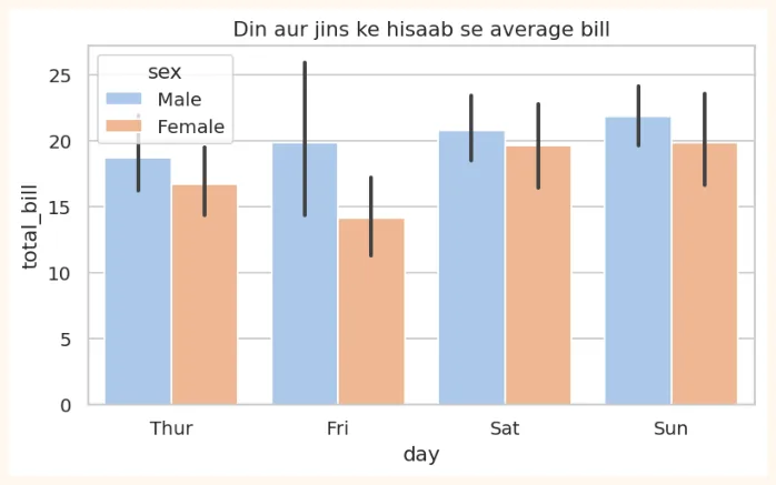
barplot har category ka average dikhata hai, aur uske upar ek kali lakeer (error bar) hoti hai jo batati hai ke ye average kitna pakka hai (confidence interval, Module 3 me).
plt.figure(figsize=(7, 3.8))
sns.barplot(data=tips, x="day", y="total_bill", hue="sex")
plt.title("Din aur jins ke hisaab se average bill")
plt.show()
OUTPUT (chart)
# barplot ke andar wohi hai jo groupby deta hai
print(tips.groupby("day", observed=True)["total_bill"].mean().round(2))
OUTPUT
day
Thur 17.68
Fri 17.15
Sat 20.44
Sun 21.41
Name: total_bill, dtype: float64
8.5 Relational Plots (do cheezon ka rishta)
scatterplot (hue, size, style ke saath)
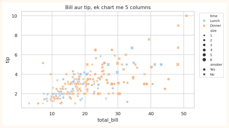
Seaborn me ek scatter plot me kai aur columns bhi dikha sakte hain: rang ( hue ), nuqte ka size ( size ), nuqte ki shakal ( style ).
plt.figure(figsize=(7.5, 4.2))
sns.scatterplot(data=tips, x="total_bill", y="tip", hue="time", size="size", style="smoker")
plt.title("Bill aur tip, ek chart me 5 columns")
plt.legend(bbox_to_anchor=(1.02, 1), loc="upper left", fontsize=8)
plt.show()
OUTPUT (chart)
regplot / lmplot (scatter + trend ki lakeer)
plt.figure(figsize=(7, 4))
sns.regplot(data=tips, x="total_bill", y="tip", line_kws={"color": "red"})
plt.title("Bill barhne par tip kaise barhti hai")
plt.show()
OUTPUT (chart)
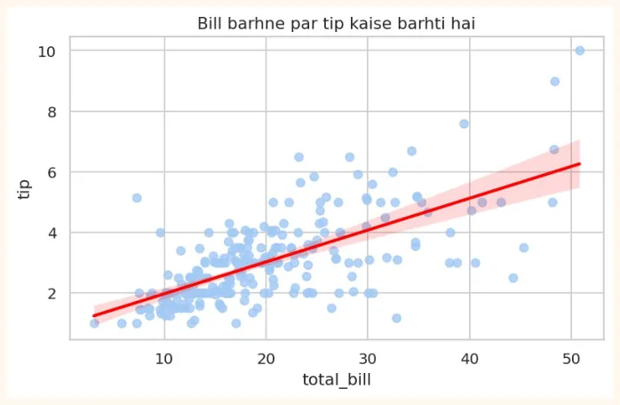
Surkh lakeer regression line hai: ye data ke beech se guzarne wali sab se behtar seedhi lakeer hai. Iske baare me Module 3 (Week 11) me poori tafseel aayegi.
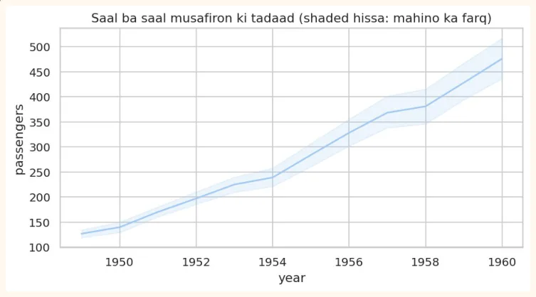
lineplot (waqt ke saath trend)
flights = sns.load_dataset("flights") # 1949 se 1960 tak mahana musafir
print(flights.head(3))
| OUTPUT | |
|---|---|
year | month passengers |
0 1949 | Jan 112 |
1 1949 | Feb 118 |
2 1949 | Mar 132 |
plt.figure(figsize=(8, 3.8))
sns.lineplot(data=flights, x="year", y="passengers")
plt.title("Saal ba saal musafiron ki tadaad (shaded hissa: mahino ka farq)")
plt.show()
OUTPUT (chart)
8.6 Heatmap aur Correlation
Correlation do numeric columns ka aapas me rishta batati hai, ek number ki shakal me jo -1 se +1 ke beech hota hai.
| Correlation | Matlab | Misaal |
|---|---|---|
| +1 | Poora sidha rishta: ek barhe to doosra bhi barhta hai | Parhne ke ghantay aur marks (taqreeban) |
| 0 | Koi rishta nahi | Joote ka size aur marks |
| -1 | Poora ulta rishta: ek barhe to doosra ghatta hai | Gari ki rafter aur safar ka waqt |
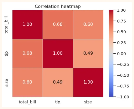
corr = tips[["total_bill", "tip", "size"]].corr()
print(corr.round(2))
OUTPUT
total_bill tip size |
|---|
total_bill 1.00 0.68 0.60 |
tip 0.68 1.00 0.49 |
size 0.60 0.49 1.00 |
Number padhna thora mushkil hai. Heatmap ye table rangon me dikhata hai: jitna gehra rang, utna mazboot rishta.
OUTPUT (chart)
-
annot=True: har dibbe me number likho.
-
cmap=: rangon ka palette (coolwarm, viridis, Blues...).
-
vmin / vmax: rang ki hadd (correlation ke liye -1 aur 1).
-
fmt=".2f": number 2 decimal tak.
BOHAT ZAROORI
Correlation ka matlab causation nahi. Garmiyon me aaiskreem ki sales aur doobne ke hadsay dono barhte hain, magar aaiskreem se koi nahi doobta. Dono ki wajah garmi hai. Correlation sirf rishta batati hai, wajah nahi.
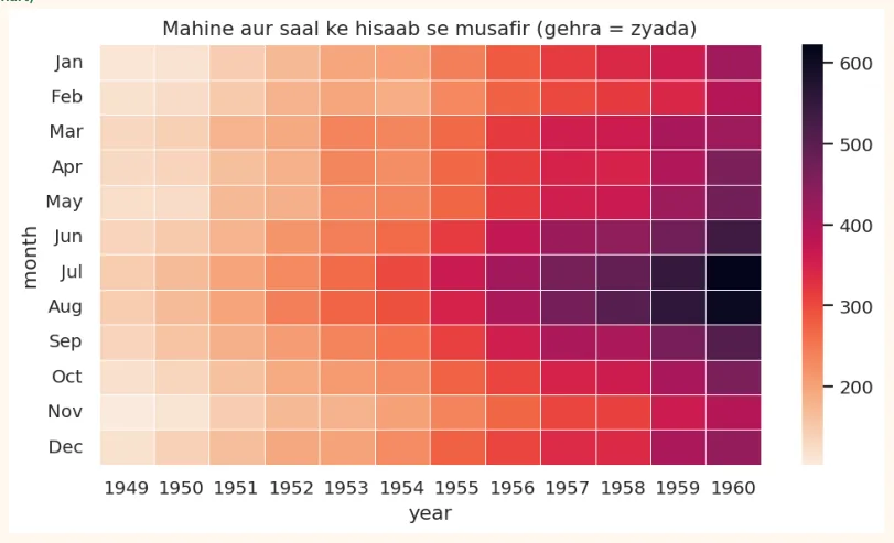
Heatmap ka doosra istemal: pivot table dikhana
pivot = flights.pivot(index="month", columns="year", values="passengers")
plt.figure(figsize=(9, 4.6))
sns.heatmap(pivot, cmap="rocket_r", linewidths=0.3)
plt.title("Mahine aur saal ke hisaab se musafir (gehra = zyada)")
plt.show()
OUTPUT (chart)
8.7 Pairplot, Jointplot aur relplot
pairplot (sab columns ka sab se muqabla)
Ek line me data ke har numeric column ka doosre se scatter plot ban jata hai, aur diagonal par har column ka histogram. Naye data ko pehli bar dekhne ke liye bohat kamal ka tool hai.
penguins = sns.load_dataset("penguins").dropna() # 3 qisam ke penguins ka data
print(penguins.shape)
sns.pairplot(penguins, hue="species", vars=["bill_length_mm", "flipper_length_mm",
"body_mass_g"],
height=2.2)
plt.show()
OUTPUT (chart)
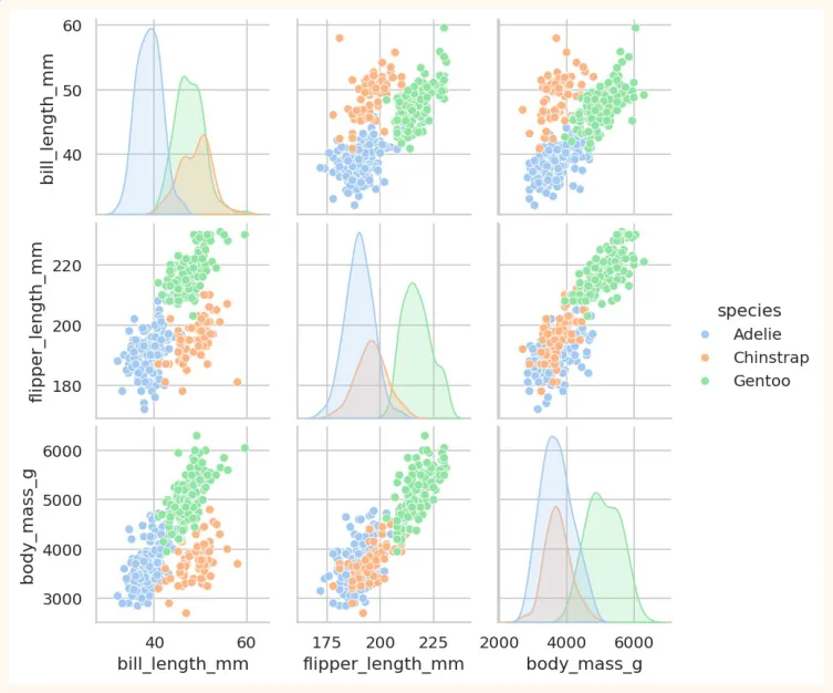
Dekho kaise teen rang (teen species) alag alag gol-gol guroohon me nazar aate hain. Ye wohi cheez hai jo ML ko classification me kaam aati hai: agar groups alag nazar aayen to model unhe asani se alag kar sakta hai.
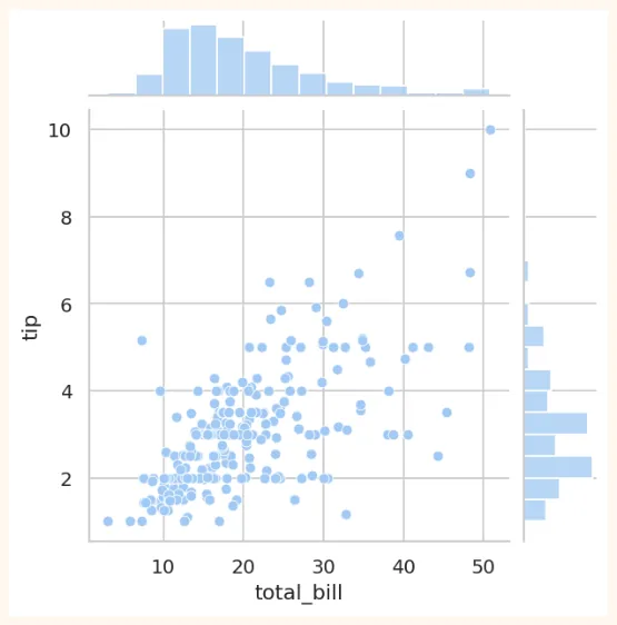
jointplot (do cheezon ka rishta aur unki apni taqseem)
sns.jointplot(data=tips, x="total_bill", y="tip", kind="scatter", height=5)
plt.show()
OUTPUT (chart)
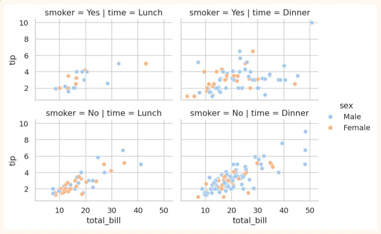
relplot / FacetGrid (har category ka alag chart)
sns.relplot(data=tips, x="total_bill", y="tip", col="time", row="smoker", hue="sex",
height=2.4, aspect=1.4)
plt.show()
OUTPUT (chart)
8.8 Seaborn ko customize aur save karna
Seaborn Matplotlib par bana hai, is liye Matplotlib ki sab cheezein (title, labels, figsize, savefig) yahan bhi chalti hain.
fig, ax = plt.subplots(figsize=(6, 3.6))
sns.boxplot(data=tips, x="time", y="tip", ax=ax, palette="Set2", hue="time", legend=False)
ax.set_title("Lunch vs Dinner: tip")
ax.set_xlabel("Waqt")
ax.set_ylabel("Tip (dollars)")
fig.savefig("tips_box.png", dpi=150, bbox_inches="tight")
print("Saved!")
OUTPUT
Saved!
AAM GALTIYAN
-
Seaborn ko x, y me column ke naam dena zaroori hai saath me data=df bhi. Sirf naam likhne se error aata hai.
-
Correlation heatmap banate waqt text columns shamil karna. Sirf numeric columns par .corr() lagao.
-
Heatmap me vmin/vmax na lagana, jis se correlation ke rang ghalat samajh aate hain.
-
Correlation ko wajah (causation) samajh lena.
-
Pairplot bohat bare data (lakhon rows) par chalana. Pehle df.sample(1000) lo.
-
Ek chart me bohat zyada cheezein (hue + size + style + col + row) daal dena. Jo samajh na aaye wo chart bekar hai.
8.9 Visualization Project: Restaurant Tips Analysis
Ab tak ke saare Matplotlib, Pandas aur Seaborn ke tools ek asli project me jodte hain. Ek restaurant ka maalik tumse poochta hai: "Mere customers kaise tip dete hain, aur kis cheez par depend karta hai?"
Project ka maqsad
-
Data ko load, inspect aur clean karna.
-
Ek naya column banana: tip_pct (bill ka kitna percent tip di gayi).
-
Kam az kam 4 sawalon ke jawab charts se dena.
-
Aakhir me insights aur recommendations likhna.
Step 1: Data load aur pehli nazar
import pandas as pd
import seaborn as sns
import matplotlib.pyplot as plt
tips = sns.load_dataset("tips")
print("Shape:", tips.shape)
print("Missing values:", tips.isnull().sum().sum())
print("Duplicates:", tips.duplicated().sum())
OUTPUT
Shape: (244, 7)
Missing values: 0
Duplicates: 1
Ek duplicate row hai. Ye ek asli data hai jahan do alag bill bilkul ek jaise ho sakte hain, is liye is project me hum ise rakhte hain. Cleaning me hamesha soch kar faisla karo.
Step 2: Naya column
tips["tip_pct"] = (tips["tip"] / tips["total_bill"] * 100).round(2)
print(tips["tip_pct"].describe().round(2))
OUTPUT
count 244.00
mean 16.08
std 6.11
min 3.56
25% 12.91
50% 15.48
75% 19.15
max 71.03
Name: tip_pct, dtype: float64
Step 3: Sawalon ke jawab (numbers se)
print("Sawal 1: smoker aur non-smoker, kis ka average tip%?")
print(tips.groupby("smoker", observed=True)["tip_pct"].mean().round(2))
print("\nSawal 2: kaunse din tip% sab se zyada?")
print(tips.groupby("day", observed=True)["tip_pct"].mean().round(2))
print("\nSawal 3: Lunch ya Dinner?")
print(tips.groupby("time", observed=True)["tip_pct"].mean().round(2))
print("\nSawal 4: table ka size aur tip%")
print(tips.groupby("size", observed=True)["tip_pct"].mean().round(2))
OUTPUT
Sawal 1: smoker aur non-smoker, kis ka average tip%?
smoker
Yes 16.32
No 15.93
Name: tip_pct, dtype: float64
Sawal 2: kaunse din tip% sab se zyada?
day
Thur 16.13
Fri 16.99
Sat 15.31
Sun 16.69
Name: tip_pct, dtype: float64
Sawal 3: Lunch ya Dinner?
time
Lunch 16.41
Dinner 15.95
Name: tip_pct, dtype: float64
Sawal 4: table ka size aur tip%
size
1 21.73
2 16.57
3 15.21
4 14.59
5 14.15
6 15.62
Name: tip_pct, dtype: float64
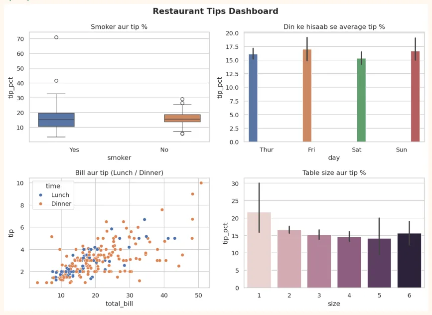
Step 4: Dashboard (4 charts ek figure me)
sns.set_theme(style="whitegrid")
fig, axes = plt.subplots(2, 2, figsize=(11, 8))
sns.boxplot(data=tips, x="smoker", y="tip_pct", hue="smoker", legend=False, ax=axes[0, 0])
axes[0, 0].set_title("Smoker aur tip %")
sns.barplot(data=tips, x="day", y="tip_pct", hue="day", legend=False, ax=axes[0, 1])
axes[0, 1].set_title("Din ke hisaab se average tip %")
sns.scatterplot(data=tips, x="total_bill", y="tip", hue="time", ax=axes[1, 0])
axes[1, 0].set_title("Bill aur tip (Lunch / Dinner)")
sns.barplot(data=tips, x="size", y="tip_pct", hue="size", legend=False, ax=axes[1, 1])
axes[1, 1].set_title("Table size aur tip %")
fig.suptitle("Restaurant Tips Dashboard", fontsize=15, fontweight="bold")
plt.tight_layout()
plt.show()
OUTPUT (chart)
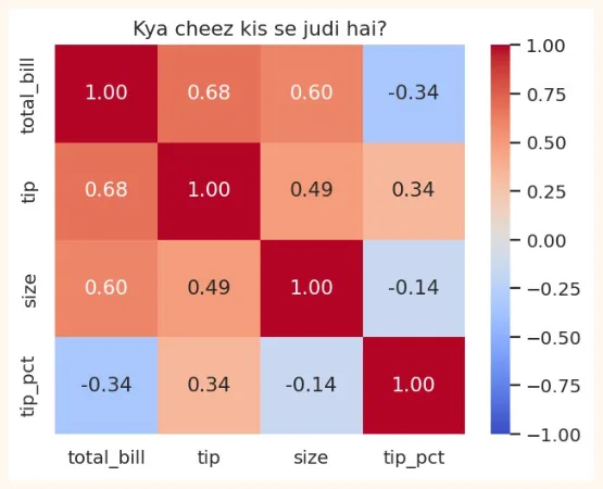
Step 5: Correlation
plt.figure(figsize=(5.5, 4.2))
sns.heatmap(tips[["total_bill", "tip", "size", "tip_pct"]].corr(), annot=True,
            cmap="coolwarm", vmin=-1, vmax=1, fmt=".2f")
plt.title("Kya cheez kis se judi hai?")
plt.show()
OUTPUT (chart)
Step 6: Insights khud likho
Charts aur numbers ko dekh kar apne alfaz me 4 se 5 jumle likho. Misaal ke taur par format:
-
Observation: "Bill barhne par tip ki raqam barhti hai (correlation mazboot hai)."
-
Lekin: "tip percent bill ke saath itna nahi barhta, yani log lagbhag ek hi percent tip dete hain."
-
Sawal ka jawab: "Smoker aur non-smoker ke tip percent me ___ farq hai." (apne output se bharo)
-
Recommendation: "Restaurant ___ par focus kare." (data se wajah ke saath)
Project ko GitHub par daalne ka tareeqa
-
Ek folder banao: tips-analysis . Is me notebook ( .ipynb ) rakho (Colab se File > Download > .ipynb).
-
Ek README.md likho: project ka naam, maqsad, dataset, tools (Pandas, Seaborn), 3 se 4 charts ke screenshots, aur insights.
-
GitHub par naya repository banao aur files upload karo.
-
Repository ka link apne CV ya LinkedIn me daalo.
8.10 Hands-on with Seaborn
Penguins dataset par practice karo (chhote chhote data science sawal):
import seaborn as sns
import matplotlib.pyplot as plt
penguins = sns.load_dataset("penguins").dropna()
print(penguins.head(3))
print(penguins["species"].value_counts())
OUTPUT
  species     island  bill_length_mm  bill_depth_mm  flipper_length_mm  \
0  Adelie  Torgersen            39.1           18.7              181.0
1  Adelie  Torgersen            39.5           17.4              186.0
2  Adelie  Torgersen            40.3           18.0              195.0
   body_mass_g     sex
0       3750.0    Male
1       3800.0  Female
2       3250.0  Female
species
Adelie       146
Gentoo       119
Chinstrap     68
Name: count, dtype: int64
-
countplot: har species ke penguins ki tadaad (aur island ke hisaab se alag rang).
-
histplot: body_mass_g ki taqseem, species ke hisaab se alag rang ( hue="species" ).
-
boxplot: flipper_length_mm species ke hisaab se. Kaunsi species ke flippers sab se lambay hain?
-
scatterplot: bill_length_mm vs bill_depth_mm, rang species ka. Kya teen groups alag nazar aate hain?
-
heatmap: penguins ke numeric columns ka correlation. Kaunse do columns me sab se mazboot rishta hai?
-
pairplot: poora dataset hue="sex" ke saath. Kya mard aur aurat penguins me farq nazar aata hai?
Bonus challenge: apna ek dataset (CSV) dhoondo (Kaggle ya koi aur) aur is chapter ke tareeqe se ek chhota visualization project banao. Ye tumhare portfolio ke liye acha pehla project hoga.
KEY TAKEAWAYS
-
Seaborn Matplotlib ke upar bana hai: kam code, khoobsurat default look, seedha DataFrame ke saath.
-
sns.set_theme() se poore notebook ka look badalta hai.
-
Distribution: histplot, kdeplot, boxplot, violinplot, stripplot. Categorical: countplot, barplot.
-
Relational: scatterplot (hue, size, style), lineplot, regplot.
-
Heatmap correlation (-1 se +1) rangon me dikhata hai. Correlation matlab causation nahi.
-
pairplot naye data ko pehli bar dekhne ka behtareen tareeqa hai. relplot/FacetGrid har category ka alag chart deta hai.
-
Insights wohi hain jo batayen ke iska matlab kya hai aur ab kya karna chahiye.