Chapter 9: Descriptive Statistics and Probability
MODULE 3 | WEEK 9
Chapter 9: Descriptive Statistics and Probability
Statistics is the science of drawing meaning from data, and Probability is the science of measuring uncertain things. Both are the soul of Data Science and Machine Learning. Every ML algorithm uses statistics and probability inside. In this chapter we will build the foundations of both with Python.
9.1 Foundations of Statistics
Statistics has two big parts:
-
Descriptive Statistics: to describe the data we have in front of us (what the average is, how spread out it is). This is the subject of this chapter.
-
Inferential Statistics: estimating things about the whole group (population) from a small amount of data (a sample). This comes in the next chapter.
Population and Sample
| Population | Sample | |
|---|---|---|
| Meaning | The whole group you want to know about | The small part of the population that we picked |
| Example | All university students in Pakistan | 500 of them who were surveyed |
| The number is called | Parameter(e.g. the population mean, mu) | Statistic(e.g. the sample mean, x-bar) |
| Why | Asking everyone is expensive or impossible | Easy, cheap, fast |
Types of data
| Type | Meaning | Example |
|---|---|---|
| Nominal (categorical) | Named categories, no order | City, colour, gender, blood group |
| Ordinal (categorical) | Categories that have an order | Grade (A, B, C), rating (1 to 5 stars), level of i |
| education | ||
| Discrete (numerical) | Whole counted numbers | Number of siblings, rooms in a house |
| Type | Meaning | Example |
|---|---|---|
| Continuous (numerical) | Any value, including decimals | Height, weight, temperature, price |
9.2 Descriptive Statistics
Let us start with a small dataset: marks of 15 students .
import numpy as np
import pandas as pd
from scipy import stats
marks = np.array([45, 52, 58, 61, 63, 65, 67, 70, 72, 75, 78, 82, 88, 95, 40])
print(marks)
print(len(marks))
OUTPUT
[45 52 58 61 63 65 67 70 72 75 78 82 88 95 40]
15
A) Central Tendency (the centre of the data)
It is a single number that represents the whole dataset. There are three ways:
| Measure | Meaning | When it is better |
|---|---|---|
| Mean(average) | Sum of all / count | When data is roughly symmetric, with no outliers |
| Median | Themiddlevalue after sorting | When there are outliers or the data is lopsided |
| Mode | The value that appears most often | For categories, or when you want the most common item |
print("Mean  :", marks.mean().round(2))
print("Median:", np.median(marks))
print("Mode  :", stats.mode(marks, keepdims=False).mode)    # if all values differ, the
smallest value
# In Pandas
s = pd.Series(marks)
print(s.mean().round(2), s.median(), s.mode().tolist()[:3])
OUTPUT
Mean  : 67.4
Median: 67.0
Mode  : 40
67.4 67.0 [40, 45, 52]
OUTPUT
Mean  : 545.0
Median: 50.0
B) Spread (how spread out the data is)
An average alone is not enough. Two classes can both average 70, but in one everyone scores between 68 and 72 and in the other between 30 and 100. This difference is measured by spread .
| Measure | Meaning | Formula / Idea |
|---|---|---|
| Range | Largest minus smallest | max - min (highly affected by outliers) |
| Variance | Average of thesquareddifferences of each value | sigma<sup>2</sup>= sum((x - mean)<sup>2</sup>) / n |
| from the mean | ||
| Standard Deviation (std) | Thesquare rootof variance (in the same units) | sigma = sqrt(variance) |
| IQR | Spread of the middle 50% of data | Q3 - Q1 (safe from outliers) |
OUTPUT
Range    : 55
Variance : 216.11
Std      : 14.7
Sample std: 15.22
Q1, Q3, IQR: 59.5 76.5 17.0
OUTPUT
Pandas std : 15.22
NumPy std  : 14.7
C) Percentiles, Quartiles and Five-number Summary
Percentile: how much of the data lies below a value. For example, the 90th percentile means 90% of students scored below that mark. Quartiles divide the data into 4 equal parts: Q1 (25%), Q2 (50%, i.e. the median), Q3 (75%).
print(np.percentile(marks, [25, 50, 75, 90]))
print(pd.Series(marks).describe().round(2))     # five-number summary + mean, std
OUTPUT
[59.5 67.  76.5 85.6]
count    15.00
mean     67.40
std      15.22
min      40.00
25%      59.50
50%      67.00
75%      76.50
max      95.00
dtype: float64
Five-number summary: Minimum, Q1, Median, Q3, Maximum. The box plot is built from it. Outliers are identified by the IQR rule (Chapter 6): values below Q1 - 1.5 x IQR or above Q3 + 1.5 x IQR .
D) Z-score (how many std a value is from the average)
Z-score = (x - mean) / std . It lets you compare things on different scales.
OUTPUT
[-1.52 -1.05 -0.64 -0.44 -0.3  -0.16 -0.03  0.18  0.31  0.52  0.72  0.99
  1.4   1.88 -1.86]
Farthest value: 95
E) Shape of data: Skewness and Kurtosis
-
Skewness (lean): close to 0 = symmetric. Positive = long tail on the right (a few very large values). Negative = long tail on the left.
-
Kurtosis: how heavy the tails of the data are. Higher kurtosis = more extreme values (outliers).
import matplotlib.pyplot as plt
np.random.seed(5)
symmetric = np.random.normal(50, 10, 1000)
right_skew = np.random.exponential(10, 1000) + 20     # tail on the right
left_skew = 100 - (np.random.exponential(10, 1000) + 20)   # tail on the left
fig, axes = plt.subplots(1, 3, figsize=(12, 3.4))
for ax, data, title in zip(axes, [symmetric, right_skew, left_skew],
                           ["Symmetric", "Right skewed (positive)", "Left skewed
(negative)"]):
    ax.hist(data, bins=30, color="#6B5B95", edgecolor="white")
    ax.axvline(data.mean(), color="red", linestyle="--", label="Mean")
    ax.axvline(np.median(data), color="green", linestyle="-", label="Median")
    ax.set_title(f"{title}\nskew = {stats.skew(data):.2f}")
    ax.legend(fontsize=8)
plt.tight_layout()
plt.show()
OUTPUT (chart)
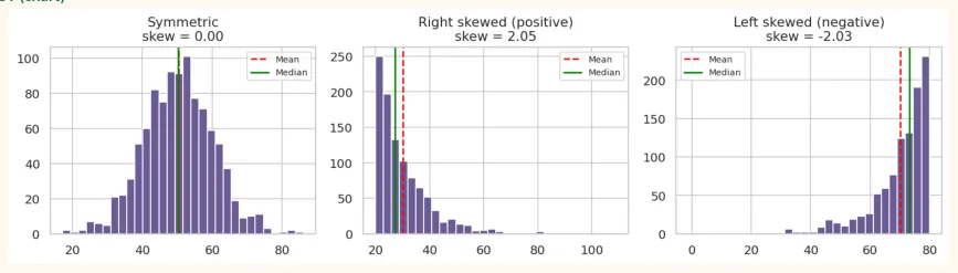
Look: in symmetric data the mean and median are in the same place. Right skewed data, the mean (red) is pulled away from the median (green) toward the right because large values drag the mean upward. Left skewed data does the opposite.
9.3 Probability Theory
Probability measures the chance of an event happening with a number between 0 and 1 . 0 means impossible, 1 means certain.
# Probability = favourable outcomes / total possible outcomes
# Probability of getting a 6 when rolling a die:
print(1 / 6)
# At least one head in two coin tosses:
print(3 / 4)
OUTPUT
0.16666666666666666
0.75
Basic terms
-
Experiment: an action whose result is not known in advance (rolling a die).
-
Sample Space (S): all possible outcomes. For a die: {1, 2, 3, 4, 5, 6}.
-
Event: any part of the sample space. "Getting an even number" = {2, 4, 6}.
-
Probability: P(event) = outcomes of the event / total outcomes (when all are equally likely).
Rules of probability
| Rule | Formula | Example |
|---|---|---|
| Complement | P(not A) = 1 - P(A) | Not getting a 6 on a die = 1 - 1/6 = 5/6 |
| Addition (or) | P(A or B) = P(A) + P(B) - P(A and B) | Drawing a heart or an ace (from a deck of cards) |
| Multiplication (and) | Independent: P(A and B) = P(A) x P(B) | Both heads on two coins = 1/2 x 1/2 = 1/4 |
| Conditional | P(A | B) = P(A and B) / P(B) |
OUTPUT
Heart or ace: 0.3077
Both aces: 0.00452
Conditional Probability and Bayes' Theorem
Conditional probability means: "if we know B has already happened, what is the probability of A?" Bayes' Theorem lets us solve the reverse question .
Bayes: P(A | B) = P(B | A) x P(A) / P(B)
OUTPUT
Probability of being sick given a positive test: 16.7 %
Only 16.7% ! The reason is that the disease is in very few people (1%), so the 5% false positives among healthy people outnumber the truly sick. This is called the base rate fallacy . This way of thinking is essential for understanding classification models in ML (spam, fraud, disease).
Permutations and Combinations (ways of counting)
-
Permutation: order matters. Choosing 2 of 3 people as "President, Vice President" (Ali-Sara and Sara-Ali are different).
-
Combination: order does not matter. A committee of 2 out of 3 people (Ali-Sara and Sara-Ali are the same).
import math
print("Permutation (3 of 5):", math.perm(5, 3))     # 5 x 4 x 3 = 60
print("Combination (3 of 5):", math.comb(5, 3))     # 10
print("Arrangements of 5 items:", math.factorial(5))    # 120
# Lottery: 6 numbers out of 49, how many ways?
print(math.comb(49, 6))
OUTPUT
Permutation (3 of 5): 60
Combination (3 of 5): 10
Arrangements of 5 items: 120
13983816
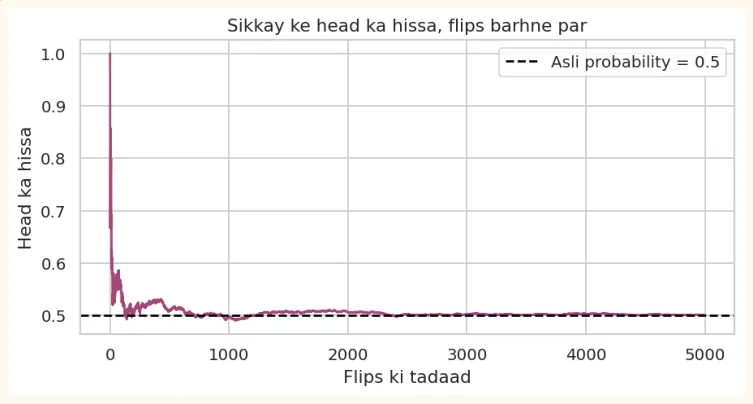
Law of Large Numbers (the law of big numbers)
The more trials you run, the closer the result gets to the true probability . Tossing a coin 10 times may give 7 heads (70%), but tossing it 10,000 times will come very close to 50%.
np.random.seed(11)
flips = np.random.randint(0, 2, 5000)                    # 1 = head
running = np.cumsum(flips) / np.arange(1, 5001)
plt.figure(figsize=(8, 3.6))
plt.plot(running, color="#A4457A")
plt.axhline(0.5, color="black", linestyle="--", label="True probability = 0.5")
plt.title("Share of heads as flips increase")
plt.xlabel("Number of flips")
plt.ylabel("Share of heads")
plt.legend()
plt.show()
OUTPUT (chart)
9.4 Random Variables and Distributions
Random variable is something whose value is decided by a random process (the result of a die, the height of a student). Probability distribution tells how likely each value is.
1) Normal Distribution (bell-shaped)
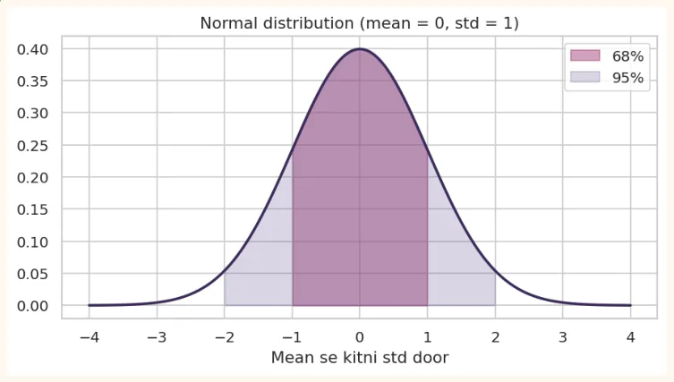
The most famous distribution. Height, weight, marks, and errors often follow it: more in the middle, fewer at both ends.
-
The mean (mu) sits in the middle and the std (sigma) decides the spread.
-
68-95-99.7 Rule: ~68% of data lies within 1 std of the mean, ~95% within 2 std, ~99.7% within 3 std.
from scipy.stats import norm
x = np.linspace(-4, 4, 400)
plt.figure(figsize=(8, 3.8))
plt.plot(x, norm.pdf(x), color="#3B2A5A", linewidth=2)
plt.fill_between(x, norm.pdf(x), where=(x > -1) & (x < 1), color="#A4457A", alpha=0.5,
label="68%")
plt.fill_between(x, norm.pdf(x), where=(x > -2) & (x < 2), color="#6B5B95", alpha=0.25,
label="95%")
plt.title("Normal distribution (mean = 0, std = 1)")
plt.xlabel("Number of std from the mean")
plt.legend()
plt.show()
OUTPUT (chart)
# Students' marks are Normal: mean = 65, std = 10
dist = norm(loc=65, scale=10)
print("P(marks < 50)      :", round(dist.cdf(50), 4))                # cdf = probability of
'less than this'
print("P(marks > 80)      :", round(1 - dist.cdf(80), 4))
print("P(55 < marks < 75) :", round(dist.cdf(75) - dist.cdf(55), 4)) # ~68%
print("Cutoff for the top 10%:", round(dist.ppf(0.90), 1))           # ppf = the reverse
question
OUTPUT
P(marks < 50)      : 0.0668
P(marks > 80)      : 0.0668
P(55 < marks < 75) : 0.6827
Cutoff for the top 10%: 77.8
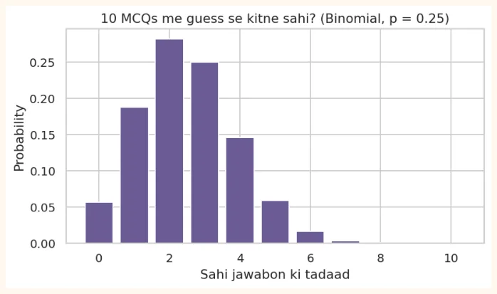
2) Binomial Distribution (counting successes / failures)
When an experiment is repeated n times , each time with only two outcomes (success/failure), and the probability of success p always stays the same. Example: a 10-question MCQ test, where the probability of guessing each one correctly is 0.25.
from scipy.stats import binom
n, p = 10, 0.25                      # 10 MCQs, 25% probability of guessing each one right
print("Exactly 3 right:", round(binom.pmf(3, n, p), 4))
print("At most 3 right:", round(binom.cdf(3, n, p), 4))
print("5 or more right:", round(1 - binom.cdf(4, n, p), 4))
print("Expected right :", n * p)
OUTPUT
Exactly 3 right: 0.2503
At most 3 right: 0.7759
5 or more right: 0.0781
Expected right : 2.5
k = np.arange(0, 11)
plt.figure(figsize=(7, 3.6))
plt.bar(k, binom.pmf(k, n, p), color="#6B5B95")
plt.title("How many of 10 MCQs right by guessing? (Binomial, p = 0.25)")
plt.xlabel("Number of correct answers")
plt.ylabel("Probability")
plt.show()
OUTPUT (chart)
3) Poisson and Uniform (brief)
-
Poisson: counts how many times an event occurs in a given time or place, when the average rate is known (calls arriving at a call centre in an hour, typos on a page).
-
Uniform: every outcome is equally likely (result of a die, random.uniform(a, b)).
from scipy.stats import poisson
# A call centre averages 4 calls/hour. Probability of exactly 6 calls?
print(round(poisson.pmf(6, mu=4), 4))
print(round(1 - poisson.cdf(7, mu=4), 4))    # 8 or more calls
OUTPUT
0.1042
0.0511
Central Limit Theorem (CLT): The biggest magic of statistics
No matter what shape the original data has (irregular, lopsided), if you repeatedly take samples from it and compute each sample's mean , then the distribution of those means becomes Normal (the larger the sample, the better). This is why the Normal distribution appears everywhere, and the confidence intervals and hypothesis tests of the next chapter stand on it.
np.random.seed(21)
population = np.random.exponential(scale=10, size=100000)     # highly skewed data
fig, axes = plt.subplots(1, 4, figsize=(13, 3.2), sharey=False)
axes[0].hist(population, bins=50, color="#B7791F")
axes[0].set_title("Original population\n(very skewed)")
for ax, n in zip(axes[1:], [2, 10, 50]):
    means = [np.random.choice(population, n).mean() for _ in range(2000)]
    ax.hist(means, bins=40, color="#6B5B95")
    ax.set_title(f"Sample means\n(n = {n})")
plt.tight_layout()
plt.show()
OUTPUT (chart)
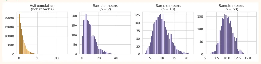
The first chart is very skewed, but as the sample size (n) grows, the distribution of means becomes bell-shaped Normal and also narrower (a more reliable estimate). That is the CLT.
9.5 Hands-on (Python Implementation)
Let us apply everything together on one dataset: the marks and study hours of 100 students in a class:
import numpy as np
import pandas as pd
from scipy import stats
np.random.seed(42)
hours = np.random.uniform(0, 10, 100).round(1)
marks = (40 + 5 * hours + np.random.normal(0, 8, 100)).clip(0, 100).round()
df = pd.DataFrame({"hours": hours, "marks": marks})
print(df.head())
print(df.describe().round(2))
OUTPUT
   hours  marks
0    3.7   59.0
1    9.5   85.0
2    7.3   77.0
3    6.0   54.0
4    1.6   46.0
        hours   marks
count  100.00  100.00
mean     4.70   63.51
std      2.97   15.54
min      0.10   34.00
25%      1.95   51.00
50%      4.65   62.50
75%      7.30   76.00
max      9.90   98.00
Exercise 1: Central tendency and spread
print("Marks mean   :", round(df["marks"].mean(), 2))
print("Marks median :", df["marks"].median())
print("Marks std    :", round(df["marks"].std(), 2))
print("IQR          :", df["marks"].quantile(0.75) - df["marks"].quantile(0.25))
print("Skewness     :", round(stats.skew(df["marks"]), 2))
OUTPUT Marks mean : 63.51 Marks median : 62.5 Marks std : 15.54 IQR : 25.0 Skewness : 0.27
Exercise 2: Find outliers with Z-score
df["z"] = stats.zscore(df["marks"])
print("Outliers (|z| > 2):", (df["z"].abs() > 2).sum())
print(df[df["z"].abs() > 2])
OUTPUT
Outliers (|z| > 2): 2
    hours  marks         z
69    9.9   96.0  2.101208
80    8.6   98.0  2.230553
Exercise 3: Probability (from data)
print("P(marks >= 70)         :", (df["marks"] >= 70).mean())
print("P(marks >= 70 | hours > 6):", round((df[df["hours"] > 6]["marks"] >= 70).mean(), 3))
OUTPUT
P(marks >= 70)         : 0.35
P(marks >= 70 | hours > 6): 0.917
Note: among students who study more than 6 hours , the probability of scoring 70+ marks is much higher than that of the whole class . This is conditional probability , and it is also a hint that studying and marks are related (which we will analyse in Week 11).
Exercise 4: Estimate with the Normal distribution
from scipy.stats import norm
m, s = df["marks"].mean(), df["marks"].std()
print("Under Normal assumption P(marks > 90):", round(1 - norm(m, s).cdf(90), 4))
print("Actual share in the data         :", (df["marks"] > 90).mean())
OUTPUT
Under Normal assumption P(marks > 90): 0.0441
Actual share in the data         : 0.06
Challenge: Solve with Binomial: if a student answers 60% of questions correctly, what is the probability of getting at least 15 right out of 20 questions? ( 1 - binom.cdf(14, 20, 0.6) )
KEY TAKEAWAYS
-
Descriptive statistics describes data; inferential statistics estimates the population from a sample.
-
Centre: mean, median, mode. Median is better with outliers. Spread: range, variance, std, IQR.
-
Use ddof=1 for std of a sample. Z-score = (x - mean) / std.
-
Skewness shows the lean of data. In right skew the mean is greater than the median.
-
Probability runs from 0 to 1. Rules: complement, addition, multiplication. Conditional and Bayes solve reverse questions.
-
In permutations order matters, in combinations it does not. Law of Large Numbers: more trials, closer to the true probability.
-
Normal (68-95-99.7), Binomial (success/failure), Poisson (event counts). CLT: the distribution of sample means becomes Normal.