Chapter 10: Inferential Statistics and Hypothesis Testing
MODULE 3 | WEEK 10
Chapter 10: Inferential Statistics and Hypothesis Testing
In the previous chapter we learned to describe data. Now the question is: whatever we see in our sample , is it also true for the whole population , or is it just luck? This question is answered by Inferential Statistics . It is used in company decisions, medical research, A/B testing and comparing ML models.
10.1 Sampling and Standard Error
We often cannot collect data from the whole population, so we take a sample If the sample is taken the wrong way, the result will be wrong too, no matter how correct the calculation is.
| Sampling method | How | Example |
|---|---|---|
| Simple Random | Everyone has an equal chance of being chosen | Putting all students' names on slips and drawing |
| Stratified | First form groups (strata), then pick randomly from each group | 50 students from each department |
| Systematic | Pick every k-th item | Every 10th student in the roll number list |
| Cluster | Pick whole groups | All students of 3 classes out of 10 |
| Convenience (bad) | Whoever is easy to reach | Asking only your friend |
WATCH OUT
Sampling bias: if a survey of "how much internet people in Pakistan use" is done only on Facebook, the result will be wrong, because people who are not online never even received the question. No matter how big the data is, a wrongly collected sample gives a wrong result.
Sampling Distribution and Standard Error
A single sample gives one mean number. If we take new samples again and again , the mean will differ slightly each time. We call the distribution of all these means the sampling distribution . Its std is called the Standard Error (SE) :
SE = s / sqrt(n) (s = sample std, n = sample size)
OUTPUT
Population mean: 60.15
One sample mean: 63.23
Mean of means : 60.19
Std of means  : 2.69
Formula 15/sqrt(30): 2.74
Look: the std of the sample means ( SE ) came out almost equal to the formula sigma / sqrt(n) . And as n increases SE falls, i.e. more data = a more reliable estimate.
10.2 Confidence Interval (CI)
Giving just one number ("the sample average is 63") is not enough. It is better to give a range in which the true population mean will probably lie. This is called a Confidence Interval .
CI = sample mean +/- (critical value x SE)
OUTPUT
Sample mean: 61.20
95% CI: (54.90, 67.51)
Why the t-distribution? When the sample is small (usually under 30) and the population std is unknown, the tdistribution is used. It is just like the Normal, only with slightly heavier tails, to include the uncertainty of a small sample. As n grows, t and Normal become the same.
The real meaning of 95% Confidence
This is the most misunderstood idea. Wrong: "the true mean is in this range with 95% probability". Correct: "if we use this method again and again repeatedly, then 95% intervals will capture the true mean". This is easy to see by running this:
import matplotlib.pyplot as plt
np.random.seed(8)
true_mean = 60
miss = 0
plt.figure(figsize=(8, 5))
for i in range(60):
    s = np.random.choice(population, 25)
    lo, hi = stats.t.interval(0.95, 24, loc=s.mean(), scale=stats.sem(s))
    hit = lo <= true_mean <= hi
    miss += (not hit)
    plt.plot([lo, hi], [i, i], color="#2F7D4F" if hit else "#C0392B", linewidth=2)
    plt.plot(s.mean(), i, "o", color="black", markersize=2.5)
True mean = 60
60 confidence intervals (red = missed the true mean, {miss} missed)
plt.xlabel("Marks")
plt.yticks([])
plt.legend()
plt.show()
OUTPUT (chart)
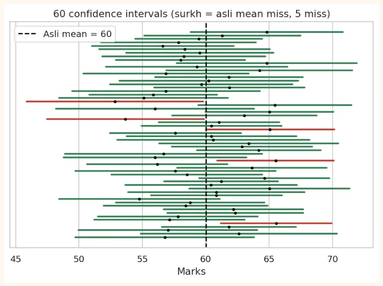
Most lines (green) capture the true mean (black line), and a few (red) miss it. A 95% CI means that over the long run about 95% of intervals capture it.
What makes a CI smaller or larger?
| Factor | Effect on CI |
|---|---|
| Sample size (n)increases | CInarrows(a more reliable estimate) |
| Spread in data (std)is higher | CIwider |
| Confidence levelincreases(95% to 99%) | CIwider(a bigger range for more certainty) |
for n in [10, 30, 100, 1000]:
    s = np.random.choice(population, n)
    lo, hi = stats.t.interval(0.95, n - 1, loc=s.mean(), scale=stats.sem(s))
    print(f"n = {n:>4}:  CI width = {hi - lo:.2f}")
OUTPUT
n =   10:  CI width = 16.23
n =   30:  CI width = 10.76
n =  100:  CI width = 6.36
n = 1000:  CI width = 1.95
10.3 Hypothesis Testing
Hypothesis testing is a method of testing a claim in the light of data.
Basic terms
| Term | Meaning | Example |
|---|---|---|
| Null Hypothesis (H0) | The default claim of "no difference / no effect" | H0: the new medicine and the old medicine have the same effect |
| Alternative (H1) | What we want to prove | H1: the new medicine has a different effect |
| Significance level (alpha) | How much error we will tolerate. Usually 0.05 (5%) | alpha = 0.05 |
| p-value | The probability of getting data this unusual (or more) if H0 is true | p = 0.01 |
How the decision is made
-
p-value < alpha (e.g. 0.01 < 0.05): the data is very unusual under H0. Reject H0 (the difference is statistically significant).
-
p-value >= alpha (e.g. 0.30): the data is consistent with H0. Cannot reject H0 (not enough evidence).
VERY IMPORTANT
What a p-value is NOT: it is not the "probability that H0 is true", nor the "probability that our result is wrong". It only answers this question: "if there were really no difference, how likely was it to see a difference this large just by chance?" . A small p-value = a small chance that it is just luck.
5 steps of a hypothesis test
-
Write H0 and H1.
-
Choose alpha (usually 0.05).
-
Choose the right test (see the table below) and compute the test statistic and p-value.
-
Compare the p-value with alpha and make the decision.
-
State the result in plain words (so that anyone can understand it without statistics).
Type I and Type II errors
| H0 is actually true | H0 is actually false | |
|---|---|---|
| H0 rejected | Type I error(false positive): punishing the innocent. Probability = alpha | Correct decision |
| H0 not rejected | Correct decision | Type II error(false negative): letting the guilty go. Probability = beta |
One-tailed vs Two-tailed
-
Two-tailed: H1 says "there is a difference" (more or less, either direction). This is what is normally used.
-
One-tailed: H1 says "it is more" or "it is less" (one direction only). Use it only when this is clear in advance.
10.4 Different Tests and Their Use
| Question | Test | scipy function |
|---|---|---|
| Is the mean of one group equal to a claimed value? | One-sample t-test | ttest_1samp |
| Is there a difference in the means of two separate groups? | Independent (two-sample) t-test | ttest_ind |
| Comparing the same group before and after? | Paired t-test | ttest_rel |
| Is there a difference in the means of three or more groups? | One-way ANOVA | f_oneway |
| Is there a relationship between two categorical variables? | Chi-square test of independence | chi2_contingency |
| Is the data Normal? | Shapiro-Wilk test | shapiro |
1) One-sample t-test
Question: a school claims its students average 60 marks. A sample gave the marks of 40 students. Is the claim correct?
np.random.seed(3)
sample = np.random.normal(64, 12, 40).round()      # marks of 40 students
t_stat, p = stats.ttest_1samp(sample, popmean=60)
print("Sample mean:", sample.mean().round(2))
print("t =", round(t_stat, 3), "| p-value =", round(p, 4))
print("Decision:", "H0 rejected (significant difference)" if p < 0.05 else "cannot reject
H0")
OUTPUT
Sample mean: 61.88
t = 0.97 | p-value = 0.3379
Decision: cannot reject H0
2) Independent two-sample t-test
Question: Are Class A's marks different from Class B's?
np.random.seed(4)
class_a = np.random.normal(68, 10, 35)
class_b = np.random.normal(62, 10, 35)
t_stat, p = stats.ttest_ind(class_a, class_b, equal_var=False)   # Welch t-test (better
default)
print("Mean A:", class_a.mean().round(2), "| Mean B:", class_b.mean().round(2))
print("t =", round(t_stat, 3), "| p-value =", round(p, 4))
print("Decision:", "H0 rejected (significant difference)" if p < 0.05 else "cannot reject
H0")
OUTPUT
Mean A: 67.3 | Mean B: 64.05
t = 1.355 | p-value = 0.1799
Decision: cannot reject H0
LESSON
An interesting point: in this data the true averages of the two classes were different (68 and 62), but because of the sample of only 35 students each, the test could not catch this difference (p-value above 0.05). This is exactly a Type II error : a real difference existed, but the evidence was not enough. With a bigger sample the difference would have been visible.
3) Paired t-test
Question: 25 students took a test before and after a training. Did the training raise their marks? (The same people, measured twice.)
np.random.seed(6)
before = np.random.normal(55, 10, 25)
after = before + np.random.normal(4, 5, 25)        # a small increase
t_stat, p = stats.ttest_rel(after, before)
print("Average increase:", (after - before).mean().round(2))
print("t =", round(t_stat, 3), "| p-value =", round(p, 4))
print("Decision:", "H0 rejected (training has an effect)" if p < 0.05 else "cannot reject
H0")
OUTPUT
Average increase: 3.28
t = 3.349 | p-value = 0.0027
Decision: H0 rejected (training has an effect)
4) One-way ANOVA (three or more groups)
Question: do the marks of students taught by three different methods differ? Running t-tests repeatedly on more than two groups is wrong (the chance of error keeps growing), so ANOVA is used.
np.random.seed(9)
method1 = np.random.normal(60, 10, 30)
method2 = np.random.normal(66, 10, 30)
method3 = np.random.normal(72, 10, 30)
f_stat, p = stats.f_oneway(method1, method2, method3)
print("F =", round(f_stat, 3), "| p-value =", round(p, 5))
print("Decision:", "At least one group is different" if p < 0.05 else "No difference
proven")
OUTPUT
F = 7.999 | p-value = 0.00065
Decision: At least one group is different
5) Chi-square test of independence (relationship between categories)
Question: is there a relationship between gender and favourite subject ? For this you need a contingency table (a count for each combination).
observed = pd.DataFrame({"Math": [30, 20], "Arts": [15, 35]},
                        index=["Male", "Female"])
print(observed)
chi2, p, dof, expected = stats.chi2_contingency(observed)
print("chi2 =", round(chi2, 3), "| p-value =", round(p, 4), "| dof =", dof)
print("Decision:", "Relationship exists" if p < 0.05 else "Relationship not proven")
OUTPUT
        Math  Arts
Male      30    15
Female    20    35
chi2 = 7.919 | p-value = 0.0049 | dof = 1
Decision: Relationship exists
6) Is the data Normal? (Shapiro-Wilk)
np.random.seed(2)
normal_data = np.random.normal(50, 5, 100)
skewed_data = np.random.exponential(5, 100)
print("Normal data p :", round(stats.shapiro(normal_data).pvalue, 4))
print("Skewed data p :", f"{stats.shapiro(skewed_data).pvalue:.2e}")
OUTPUT
Normal data p : 0.5678
Skewed data p : 1.22e-08
Here H0 = the data is Normal . A small p-value (< 0.05) means the data is not Normal. For t-tests and ANOVA (especially in small samples) it is good for the data to be approximately Normal. If it is not, non-parametric tests are used (such as Mann-Whitney U, stats.mannwhitneyu ).
10.5 A/B Testing
A/B testing is the most common hypothesis test in companies: run two versions (A and B) on two random groups and see whether there is a real difference.
OUTPUT
Rate A: 0.1 | Rate B: 0.125
z = -2.502 | p-value = 0.0124
Decision: B difference is significant
10.6 Common mistakes and important cautions
-
Statistical significance is not practical importance: in a very large sample even a tiny difference can come out "significant" (e.g. a 0.1 difference in average marks). Look not just at the p-value but also at the size of the difference (effect size) .
-
p-hacking: running lots of tests and reporting only the ones that came out "significant". Run 20 tests and one will come under 0.05 by chance.
-
H0 is never "proven": "cannot reject H0" does not mean "H0 is true". It only means the evidence was not enough.
-
Test assumptions: every test has conditions (Normal data, independence). Do not apply a test without checking them.
-
Correlation vs causation: only a randomized experiment (like an A/B test) can prove causation.
A short look at effect size (Cohen's d)
def cohens_d(a, b):
na, nb = len(a), len(b)
    pooled = np.sqrt(((na - 1) * a.std(ddof=1) ** 2 + (nb - 1) * b.std(ddof=1) ** 2) / (na +
nb - 2))
return (a.mean() - b.mean()) / pooled
print("Cohen's d (class A vs B):", round(cohens_d(class_a, class_b), 2))
# Rule of thumb: 0.2 small, 0.5 medium, 0.8 large difference
OUTPUT
Cohen's d (class A vs B): 0.32
10.7 Hands-on
Create the data below and answer the questions:
np.random.seed(100)
men = np.random.normal(172, 7, 50)        # heights of men (cm)
women = np.random.normal(160, 6, 50)      # heights of women (cm)
print(men.mean().round(1), women.mean().round(1))
OUTPUT
171.7 159.0
Exercise 1: Confidence Interval
lo, hi = stats.t.interval(0.95, len(men) - 1, loc=men.mean(), scale=stats.sem(men))
print(f"95% CI of men's height: ({lo:.1f}, {hi:.1f})")
OUTPUT
95% CI of men's height: (169.8, 173.6)
Exercise 2: One-sample test
Is the average height of men 170 cm? (H0: mu = 170)
t, p = stats.ttest_1samp(men, 170)
print("p-value:", round(p, 4), "->", "H0 rejected" if p < 0.05 else "H0 not rejected")
OUTPUT
p-value: 0.0746 -> H0 not rejected
Exercise 3: Two-sample test and effect size
t, p = stats.ttest_ind(men, women, equal_var=False)
print("p-value:", p)
print("Cohen's d:", round(cohens_d(men, women), 2))
OUTPUT
p-value: 1.2012679922177802e-16
Cohen's d: 2.0
Exercise 4: A/B test
For email subject line A, 120 out of 1000 people opened the email, and for B, 150 out of 1000 did. Decide using proportions_ztest and write your conclusion in two sentences.
z, p = proportions_ztest(np.array([120, 150]), np.array([1000, 1000]))
print("p-value:", round(p, 4))
OUTPUT
p-value: 0.0496
Note: the p-value is very close to 0.05. It is hard to decide at such a boundary. It is better to rerun the test on more visitors or also look at the effect size and CI, and not rely only on the word "significant".
KEY TAKEAWAYS
-
Inferential statistics estimates the population from a sample. The sampling method must be correct (random).
-
Standard Error = s / sqrt(n). Increasing the sample size reduces SE and improves the estimate.
-
95% Confidence Interval means: if you repeat this method many times, 95% of the intervals capture the true value.
-
Hypothesis test: H0 (no difference) and H1. If p-value < alpha (0.05), reject H0. The p-value is not the probability that H0 is true.
-
Type I = false alarm (alpha). Type II = alarm failing to ring (beta).
-
Tests: ttest_1samp, ttest_ind (Welch), ttest_rel (paired), f_oneway (ANOVA), chi2_contingency, shapiro.
-
Significance and practical importance are different: always look at the effect size. Avoid p-hacking.