Chapter 11: Linear Regression and Regression Project
MODULE 3 | WEEK 11
Chapter 11: Linear Regression and Regression Project
So far we have described data and tested claims. Now the biggest step: prediction . Linear Regression is the very first and most widely used algorithm of machine learning. Once you understand it, many later ML algorithms will feel easy. First Covariance and Correlation (the relationship between two things), then regression, and finally a complete project.
11.1 Covariance and Correlation
Do two things change together? For example, when study hours increase, do marks increase too? There are two ways to measure this relationship.
Covariance
Covariance tells whether two things change together or not, and in which direction .
-
Positive covariance: if one rises, the other rises too.
-
Negative covariance: if one rises, the other falls.
-
Near zero: no straight-line relationship.
The problem is that the covariance number depends on units (measure height in cm or in metres and the number changes), so by reading it we cannot tell "how strong the relationship is". The solution to this problem is correlation .
Correlation (Pearson r)
Correlation = covariance / (std of x x std of y) . It standardizes the covariance, so it always stays between -1 and +1 and the effect of units disappears.
| Value of r | Meaning |
|---|---|
| +0.7 to +1 | Strong positive relationship |
| +0.3 to +0.7 | Moderate positive relationship |
| -0.3 to +0.3 | Weak or no (linear) relationship |
| -0.7 to -0.3 | Moderate negative relationship |
| -1 to -0.7 | Strong negative relationship |
import numpy as np
import pandas as pd
from scipy import stats
import matplotlib.pyplot as plt
np.random.seed(42)
hours = np.random.uniform(0, 10, 80)
marks = 40 + 5 * hours + np.random.normal(0, 8, 80)
print("Covariance:", np.cov(hours, marks)[0, 1].round(2))
print("Correlation:", np.corrcoef(hours, marks)[0, 1].round(3))
df = pd.DataFrame({"hours": hours, "marks": marks})
print(df.corr().round(3))
OUTPUT
Covariance: 50.08
Correlation: 0.906
       hours  marks
hours  1.000  0.906
marks  0.906  1.000
Pearson vs Spearman
-
Pearson: only a measures straight-line (linear) relationships.
-
Spearman: works on the ranking (order) of values, so it measures every steadily increasing (or decreasing) relationship (monotonic) (straight or not) and is less affected by outliers.
x = np.arange(1, 21)
y = x ** 3                               # increases, but not in a straight line
print("Pearson :", round(stats.pearsonr(x, y)[0], 3))
print("Spearman:", round(stats.spearmanr(x, y)[0], 3))      # exactly 1.0
OUTPUT
Pearson : 0.922
Spearman: 1.0
Pictures of different relationships
np.random.seed(0)
n = 100
x = np.random.normal(0, 1, n)
cases = {
    "r = +0.9": 0.9 * x + np.random.normal(0, 0.45, n),
    "r = +0.5": 0.5 * x + np.random.normal(0, 0.87, n),
    "r = 0": np.random.normal(0, 1, n),
    "r = -0.5": -0.5 * x + np.random.normal(0, 0.87, n),
    "r = -0.9": -0.9 * x + np.random.normal(0, 0.45, n),
    "A relationship, but r ~ 0": x ** 2 + np.random.normal(0, 0.2, n),
}
fig, axes = plt.subplots(2, 3, figsize=(10, 6))
for ax, (title, y) in zip(axes.ravel(), cases.items()):
    ax.scatter(x, y, s=12, color="#6B5B95", alpha=0.7)
    ax.set_title(f"{title}  (actual r = {np.corrcoef(x, y)[0, 1]:.2f})", fontsize=10)
plt.tight_layout()
plt.show()
OUTPUT (chart)
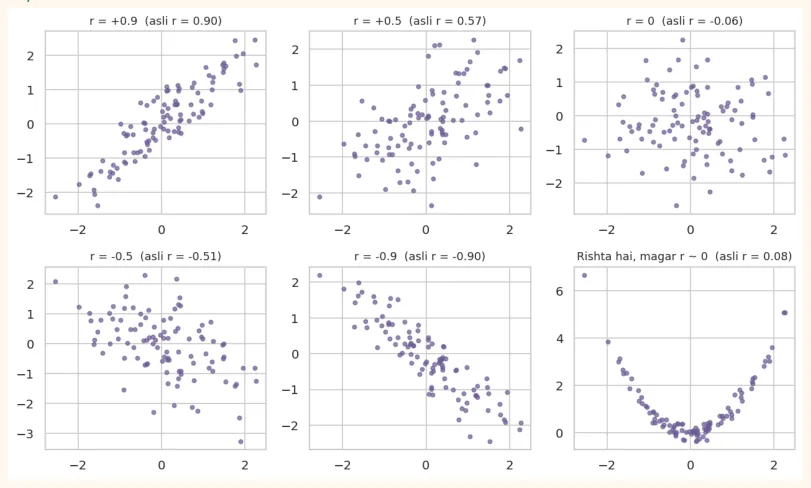
The last chart is a very important lesson: x and y have a clear relationship (U-shape), but Pearson r is almost 0 , because it is not a straight-line relationship . So do not trust the number alone; always look at the scatter plot too.
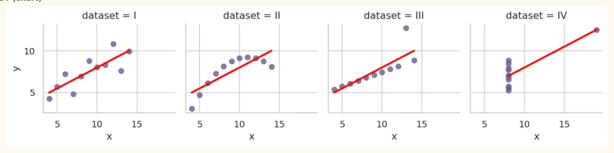
Anscombe's Quartet: four datasets, identical numbers
The statistician Francis Anscombe created four different datasets whose mean, variance, correlation and regression line are exactly the same , yet the pictures are completely different.
import seaborn as sns
anscombe = sns.load_dataset("anscombe")
summary = anscombe.groupby("dataset").agg(
x_mean=("x", "mean"), y_mean=("y", "mean"), y_std=("y", "std"))
summary["corr"] = anscombe.groupby("dataset").apply(lambda d: d["x"].corr(d["y"]),
include_groups=False)
print(summary.round(2))
OUTPUT
         x_mean  y_mean  y_std  corr
dataset
I           9.0     7.5   2.03  0.82
II          9.0     7.5   2.03  0.82
III         9.0     7.5   2.03  0.82
IV          9.0     7.5   2.03  0.82
sns.lmplot(data=anscombe, x="x", y="y", col="dataset", col_wrap=4, height=2.6,
           ci=None, scatter_kws={"color": "#6B5B95"}, line_kws={"color": "red"})
plt.show()
OUTPUT (chart)
LESSON FROM ANSCOMBE
The numbers of all four are the same, but the first is fine, the second is curved, in the third an outlier is pulling the line, and in the fourth everything rests on a single point. Lesson: always plot the data before modelling.
11.2 Simple Linear Regression
Simple Linear Regression uses one input (x) to predict one output (y) , by drawing a straight line through the data:
y = b0 + b1 x
-
y: the thing we want to predict (target / dependent variable), e.g. marks.
-
x: what we predict from (feature / independent variable), e.g. study hours.
-
b1 (slope): how much y changes when there is a 1-unit increase in x.
-
b0 (intercept): what y will be when x = 0.
Which is the best line? (Least Squares)
Thousands of lines can pass through the data. Best is the one that makes the sum of squared errors (residuals) the smallest. Residual = actual y - predicted y (i.e. how far each point is from the line).
np.random.seed(5)
x = np.random.uniform(1, 10, 15)
y = 35 + 6 * x + np.random.normal(0, 7, 15)
b1, b0 = np.polyfit(x, y, 1)
pred = b0 + b1 * x
plt.figure(figsize=(7.5, 4.2))
plt.scatter(x, y, color="#6B5B95", s=45, zorder=3, label="Actual data")
xs = np.linspace(0, 11, 50)
plt.plot(xs, b0 + b1 * xs, color="red", linewidth=2, label="Best-fit line")
for xi, yi, pi in zip(x, y, pred):
    plt.plot([xi, xi], [yi, pi], color="gray", linestyle=":", linewidth=1)   # residual
plt.title("Short dotted lines = residuals (errors)")
plt.xlabel("Study hours (x)")
plt.ylabel("Marks (y)")
plt.legend()
plt.show()
OUTPUT (chart)
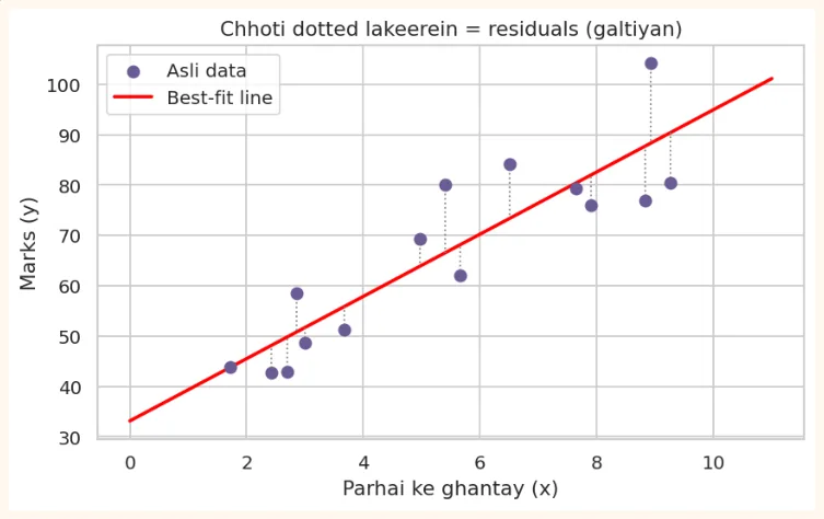
Formula for slope and intercept
b1 = covariance(x, y) / variance(x) and b0 = mean(y) - b1 x mean(x) . Let us compute it three ways:
# 1) By hand (formula)
b1_manual = np.cov(x, y, ddof=1)[0, 1] / np.var(x, ddof=1)
b0_manual = y.mean() - b1_manual * x.mean()
print("Manual   :", round(b1_manual, 3), round(b0_manual, 3))
# 2) NumPy polyfit (degree 1 = straight line)
b1_np, b0_np = np.polyfit(x, y, 1)
print("polyfit  :", round(b1_np, 3), round(b0_np, 3))
# 3) SciPy linregress (also gives r and p-value)
res = stats.linregress(x, y)
print("linregress:", round(res.slope, 3), round(res.intercept, 3),
      "| r =", round(res.rvalue, 3), "| p =", f"{res.pvalue:.2e}")
OUTPUT
Manual   : 6.182 33.15
polyfit  : 6.182 33.15
linregress: 6.182 33.15 | r = 0.883 | p = 1.28e-05
All three methods gave the same answer. This gives us the line hidden in the data, y = b0 + b1 x .
Interpretation (what the result means)
print(f"Marks = {res.intercept:.1f} + {res.slope:.1f} x hours")
print("Slope:", round(res.slope, 2), "-> marks rise by about this much for each extra hour")
print("Intercept:", round(res.intercept, 1), "-> predicted marks for 0 hours of study")
new_hours = 8
print(f"Prediction for {new_hours} hours:", round(res.intercept + res.slope * new_hours, 1))
OUTPUT
Marks = 33.1 + 6.2 x hours
Slope: 6.18 -> marks rise by about this much for each extra hour
Intercept: 33.1 -> predicted marks for 0 hours of study
Prediction for 8 hours: 82.6
COMMON MISTAKES
-
Extrapolation: predicting outside the range of the data (e.g. 1 to 10 hours). At 100 hours you would get "marks = 600", which is meaningless. The model is reliable only within the range it was built on.
-
Always treating the intercept as meaningful. When x = 0 is not even possible (such as height 0), the intercept has no real meaning.
-
Mistaking the slope for a cause . Regression shows a relationship; it does not prove causation.
R-squared (R<sup>2</sup> ): how good is the model?
R<sup>2</sup> = 1 - (sum of squared residuals) / (total spread) . It means: the share of the spread in y that the model can explain .
-
R<sup>2</sup> = 0.8 means that of the variation in marks, 80% can be explained by study hours.
-
R<sup>2</sup> = 0 means the model is no better than the average. R<sup>2</sup> = 1 means perfectly correct.
-
In simple regression R<sup>2</sup> = r<sup>2</sup> (the square of the correlation).
pred = res.intercept + res.slope * x
ss_res = ((y - pred) ** 2).sum()           # sum of squared residuals
ss_tot = ((y - y.mean()) ** 2).sum()       # total spread
r2 = 1 - ss_res / ss_tot
print("R-squared:", round(r2, 3), "| r**2:", round(res.rvalue ** 2, 3))
OUTPUT
R-squared: 0.78 | r**2: 0.78
11.3 statsmodels: the full regression report
In Data Science, it is important to know not only the prediction but also how reliable each coefficient is . statsmodels library gives a complete statistical report. The Formula API ("y ~ x") is as easy as in the R language.
import statsmodels.formula.api as smf
np.random.seed(42)
hours = np.random.uniform(0, 10, 100)
marks = 40 + 5 * hours + np.random.normal(0, 8, 100)
df = pd.DataFrame({"hours": hours, "marks": marks})
model = smf.ols("marks ~ hours", data=df).fit()
print(model.summary())
OUTPUT
OLS Regression Results
==============================================================================
Dep. Variable:                  marks   R-squared:                       0.785
Model:                            OLS   Adj. R-squared:                  0.782
Method:                 Least Squares   F-statistic:                     356.9
Date:                Tue, 13 Oct 2026   Prob (F-statistic):           1.95e-34
Time:                        11:52:00   Log-Likelihood:                -339.09
No. Observations:                 100   AIC:                             682.2
Df Residuals:                      98   BIC:                             687.4
Df Model:                           1
Covariance Type:            nonrobust
==============================================================================
                 coef    std err          t      P>|t|      [0.025      0.975]
------------------------------------------------------------------------------
Intercept     41.7208      1.362     30.625      0.000      39.017      44.424
hours          4.6322      0.245     18.892      0.000       4.146       5.119
==============================================================================
Omnibus:                        0.900   Durbin-Watson:                   2.285
Prob(Omnibus):                  0.638   Jarque-Bera (JB):                0.808
Skew:                           0.217   Prob(JB):                        0.668
Kurtosis: 2.929 Cond. No. 10.7
==============================================================================
Notes:
[1] Standard Errors assume that the covariance matrix of the errors is correctly sp...
How to read the report
| Part | Meaning |
|---|---|
| R-squared | How much of the spread in marks the model explained |
| Adj. R-squared | The form of R-squared that penalizes useless features (important in multiple regression) |
| coef(Intercept, hours) | b0 and b1 (the effect of each x) |
| std err | The standard error of the coefficient: how uncertain the estimate is |
| **t and P> | t |
| [0.025, 0.975] | The 95% confidence interval of the coefficient |
| F-statistic, Prob (F) | Whether the whole model is useful (does at least one x have an effect?) |
See how everything from the previous chapters (hypothesis test, p-value, confidence interval) comes together in one place here. This is what ties it all together.
print("Coefficients:")
print(model.params.round(3))
print("\nP-values:")
print(model.pvalues.round(4))
print("\n95% CI:")
print(model.conf_int().round(3))
print("\nR-squared:", round(model.rsquared, 3))
OUTPUT
Coefficients:
Intercept    41.721
hours         4.632
dtype: float64
P-values:
Intercept    0.0
hours        0.0
dtype: float64
95% CI:
                0       1
Intercept  39.017  44.424
hours       4.146   5.119
R-squared: 0.785
# Prediction on new data
new = pd.DataFrame({"hours": [2, 5, 9]})
print(model.predict(new).round(1))
OUTPUT
0    51.0
1    64.9
2    83.4
dtype: float64
11.4 Multiple Linear Regression
In real life one thing (y) depends on many factors. Multiple Linear Regression has several inputs:
y = b0 + b1 x1 + b2 x2 + ... + bk xk
OUTPUT
        price         size  bedrooms        age       city
0  373.428765   728.924868         1   6.433031     Lahore
1  621.493903  2839.756377         3  29.361627     Lahore
2  531.945474  1815.227694         5  32.316518     Lahore
3  986.987204  2670.395533         3  27.956046  Islamabad
4  472.921537  3433.968536         5  38.593854    Karachi
m2 = smf.ols("price ~ size + bedrooms + age + C(city)", data=houses).fit()
print(m2.params.round(3))
print("R-squared:", round(m2.rsquared, 3), "| Adj R-squared:", round(m2.rsquared_adj, 3))
OUTPUT
Intercept | 601.643 |
|---|---|
C(city)[T.Karachi] | -594.459 |
C(city)[T.Lahore] | -386.205 |
size | 0.129 |
bedrooms | 40.920 |
age | -3.933 |
dtype: float64 | |
| `R-squared: 0.955 | ` |
The model found numbers close to the true coefficients : the effect of size ~0.12, bedrooms ~40, age ~-4. C(city) automatically turned the city into dummy variables (0/1 columns). The city that comes first alphabetically ( Islamabad ) became the base category , so the coefficients of Karachi and Lahore show the difference compared to Islamabad : Karachi about -600 and Lahore about -400, which match the differences in our true formula (Islamabad +600, Lahore +200, Karachi 0).
How to read a coefficient
In multiple regression each coefficient means: holding everything else equal , the change in y for a 1-unit increase in this x. For example, size 0.12 means if the number of rooms, age and city are the same , then each extra square foot raises the price by about 0.12 lakh.
Why Adjusted R-squared?
The more features you add, R<sup>2</sup> only goes up (even if the feature is useless). Adjusted R<sup>2</sup> penalizes useless features, so it is better for comparing models.
Multicollinearity (when features are highly related to each other)
If two inputs are highly correlated with each other (such as size in sq ft and size in sq meter ) the model cannot decide which one has the effect, and the coefficients become unreliable. First look at the correlation matrix , and also check the VIF (Variance Inflation Factor; be suspicious if above 5).
from statsmodels.stats.outliers_influence import variance_inflation_factor
X = houses[["size", "bedrooms", "age"]].copy()
X.insert(0, "const", 1.0)
vif = pd.Series([variance_inflation_factor(X.values, i) for i in range(1, X.shape[1])],
                index=["size", "bedrooms", "age"])
print(vif.round(2))          # fine if all are below 5
OUTPUT
size        1.01
bedrooms    1.01
age         1.01
dtype: float64
11.5 Regression assumptions and Residual Plots
Linear regression is reliable when the data meets some conditions. An easy way to remember them: LINE .
| Assumption | How to check | |
|---|---|---|
| L | **Linearity:**the relationship between x and y is like a straight line | Scatter plot; no curve in the residuals vs fitted plot |
| I | **Independence:**each observation is independent of the others | How the data was collected (can be a problem in time series) |
| N | **Normality:**residuals are roughly Normal | Histogram and Q-Q plot of residuals |
| E | **Equal variance:**the spread of residuals is the same everywhere (homoscedasticity) | Residuals vs fitted: an evenly wide band-like pattern throughout |
import statsmodels.api as sm
fitted = m2.fittedvalues
resid = m2.resid
fig, axes = plt.subplots(1, 3, figsize=(13, 3.8))
axes[0].scatter(fitted, resid, color="#6B5B95", alpha=0.6, s=18)
axes[0].axhline(0, color="red", linestyle="--")
axes[0].set_title("Residuals vs Fitted\n(no pattern = good)")
axes[0].set_xlabel("Fitted values")
axes[0].set_ylabel("Residuals")
axes[1].hist(resid, bins=20, color="#A4457A", edgecolor="white")
axes[1].set_title("Histogram of residuals\n(bell-shaped = good)")
sm.qqplot(resid, line="45", fit=True, ax=axes[2], markerfacecolor="#6B5B95", markersize=3)
axes[2].set_title("Q-Q plot\n(points on the line = Normal)")
plt.tight_layout()
plt.show()
OUTPUT (chart)
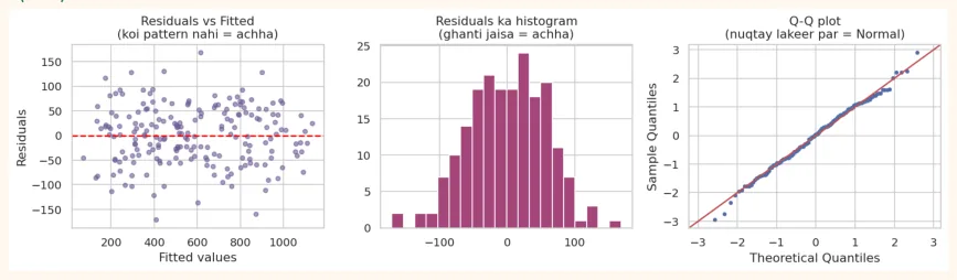
All three plots show a healthy situation. Now see what happens when the relationship is not a straight line and we still fit a straight line:
np.random.seed(3)
xc = np.random.uniform(0, 10, 100)
yc = 3 + 0.5 * xc ** 2 + np.random.normal(0, 3, 100)          # curved relationship
bad = smf.ols("y ~ x", data=pd.DataFrame({"x": xc, "y": yc})).fit()
fig, axes = plt.subplots(1, 2, figsize=(10, 3.8))
axes[0].scatter(xc, yc, color="#6B5B95", s=15)
axes[0].plot(np.sort(xc), bad.predict(pd.DataFrame({"x": np.sort(xc)})), color="red")
axes[0].set_title("The straight line is not capturing the curve")
axes[1].scatter(bad.fittedvalues, bad.resid, color="#A4457A", s=15)
axes[1].axhline(0, color="black", linestyle="--")
axes[1].set_title("U-shape pattern in residuals = Linearity fails")
plt.tight_layout()
plt.show()
OUTPUT (chart)
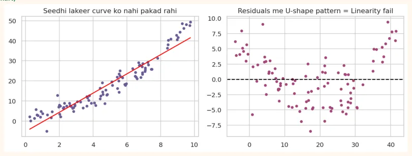
The residuals show a clear U-shape pattern , which shows that a straight line is the wrong model for this data. Fix: add x squared ( x ** 2 ) (polynomial regression), or apply a log transform , or use another algorithm (Decision Tree, Random Forest), which come in later modules.
11.6 Evaluation Metrics and Train/Test Split
Testing a model on the same data it learned from is cheating . It is as if you memorized the exact questions that would come in the paper before the exam and scored well, but what happens with new questions? That is why we split the data into two parts:
-
Train set (usually 80%): the model learns from this.
-
Test set (20%): the model has never seen this. Real performance is measured on this.
| Metric | Formula / Idea | Meaning |
|---|---|---|
| MAE | Mean Absolute Error: average of | actual - predicted |
| Metric | Formula / Idea | Meaning |
|---|---|---|
| MSE | Mean Squared Error: (actual - predicted)<sup>2</sup>differences of each value from the mean | Punishes large errors more |
| RMSE | sqrt(MSE) | Like MSE but in original units, the most common |
| R<sup>2</sup> | 1 - SSres / SStot | How much of the spread the model explained (closer to 1 is better) |
from sklearn.model_selection import train_test_split
from sklearn.linear_model import LinearRegression
from sklearn.metrics import mean_absolute_error, mean_squared_error, r2_score
X = pd.get_dummies(houses[["size", "bedrooms", "age", "city"]], drop_first=True)
y = houses["price"]
X_train, X_test, y_train, y_test = train_test_split(X, y, test_size=0.2, random_state=42)
print("Train:", X_train.shape, "| Test:", X_test.shape)
model_sk = LinearRegression().fit(X_train, y_train)
pred = model_sk.predict(X_test)
print("MAE :", round(mean_absolute_error(y_test, pred), 2))
print("RMSE:", round(np.sqrt(mean_squared_error(y_test, pred)), 2))
print("R2 (test) :", round(r2_score(y_test, pred), 3))
print("R2 (train):", round(model_sk.score(X_train, y_train), 3))
OUTPUT
Train: (160, 5) | Test: (40, 5)
MAE : 56.39
RMSE: 71.14
R2 (test) : 0.931
R2 (train): 0.961
DIFFERENCE BETWEEN THE TWO
In this chapter we saw both statsmodels (statistics: p-values, interpretation) and scikit-learn (machine learning: prediction, train/test). The nature of statistics is to understand , the nature of ML is to predict . Both are needed.
11.7 Regression Model Project: Car Fuel Efficiency (mpg)
Question: predict a car's fuel efficiency (mpg: miles per gallon) from its characteristics (weight, horsepower, model year, etc.), and understand which factor affects efficiency the most. Data: 398 cars (seaborn's mpg dataset).
Step 1: Load and inspect the data
import seaborn as sns
import pandas as pd
import numpy as np
import matplotlib.pyplot as plt
import statsmodels.formula.api as smf
cars = sns.load_dataset("mpg")
print(cars.shape)
print(cars.isnull().sum()[cars.isnull().sum() > 0])
print(cars.head(3))
OUTPUT
(398, 9)
horsepower    6
dtype: int64
    mpg  cylinders  displacement  horsepower  weight  acceleration  \
0  18.0          8         307.0       130.0    3504          12.0
1  15.0          8         350.0       165.0    3693          11.5
2  18.0          8         318.0       150.0    3436          11.0
   model_year origin                       name
0          70    usa  chevrolet chevelle malibu
1          70    usa          buick skylark 320
2          70    usa         plymouth satellite
Step 2: Cleaning
horsepower has 6 missing values. Only 6 rows (1.5%), so dropping them is fine.
cars = cars.dropna().reset_index(drop=True)
print(cars.shape)
print(cars[["mpg", "weight", "horsepower", "acceleration",
"model_year"]].describe().round(1))
OUTPUT
(392, 9)
         mpg  weight  horsepower  acceleration  model_year
count  392.0   392.0       392.0         392.0       392.0
mean    23.4  2977.6       104.5          15.5        76.0
std      7.8   849.4        38.5           2.8         3.7
min      9.0  1613.0        46.0           8.0        70.0
25%     17.0  2225.2        75.0          13.8        73.0
50%     22.8  2803.5        93.5          15.5        76.0
75%     29.0  3614.8       126.0          17.0        79.0
max     46.6  5140.0       230.0          24.8        82.0
Step 3: EDA
fig, axes = plt.subplots(1, 3, figsize=(13, 3.8))
sns.histplot(cars["mpg"], bins=25, kde=True, ax=axes[0], color="#6B5B95")
axes[0].set_title("Distribution of mpg")
sns.scatterplot(data=cars, x="weight", y="mpg", hue="origin", ax=axes[1])
axes[1].set_title("Weight and mpg")
sns.heatmap(cars[["mpg", "cylinders", "displacement", "horsepower", "weight",
"acceleration", "model_year"]].corr(),
            annot=True, fmt=".2f", cmap="coolwarm", vmin=-1, vmax=1, ax=axes[2],
annot_kws={"size": 7})
axes[2].set_title("Correlation")
plt.tight_layout()
plt.show()
OUTPUT (chart)
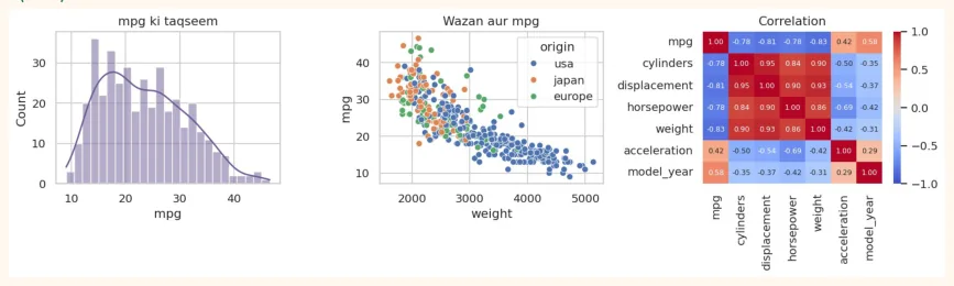
Observations: The relationship of mpg with weight is strongly negative (heavy car = low mileage). displacement, horsepower, cylinders and weight are also highly correlated with each other (a multicollinearity risk). The relationship is not a perfect straight line; it is slightly curved.
Step 4: Model 1, weight only
m1 = smf.ols("mpg ~ weight", data=cars).fit()
print(m1.params.round(4))
print("R-squared:", round(m1.rsquared, 3))
print("Change in mpg for every 1000 lb increase in weight:", round(m1.params["weight"] *
1000, 2))
OUTPUT
Intercept    46.2165
weight       -0.0076
dtype: float64
R-squared: 0.693
Change in mpg for every 1000 lb increase in weight: -7.65
Step 5: Model 2, several features
m2 = smf.ols("mpg ~ weight + horsepower + acceleration + model_year + C(origin)",
data=cars).fit()
print(m2.summary().tables[1])
print("R-squared:", round(m2.rsquared, 3), "| Adj R-squared:", round(m2.rsquared_adj, 3))
OUTPUT
|===============================coef-------------------------------|=======================================================std err t P>|t| [0.025 0.975]-------------------------------------------------------|
|---|---|
|Intercept -16.0654|4.562 -3.522 0.000 -25.035 -7.096|
|C(origin)[T.japan] 0.3326|0.569 0.585 0.559 -0.785 1.451|
|C(origin)[T.usa] -1.9363|0.521 -3.715 0.000 -2.961 -0.912|
|weight -0.0057|0.001 -11.252 0.000 -0.007 -0.005|
|horsepower -0.0048|0.013 -0.360 0.719 -0.031 0.021|
|acceleration 0.0392|0.098 0.401 0.689 -0.153 0.231|
|model_year 0.7554===============================|0.052 14.617 0.000 0.654 0.857=======================================================|
|R-squared: 0.819 | Adj R-square|d: 0.817|
p-values : features whose p-value is above 0.05 (such as acceleration and horsepower ) their effect, together with the other factors, is not proven , because weight and model_year already explain most of the effect. weight and model_year have a strong effect (the positive coefficient of model_year shows that cars from newer years are more fuel-efficient).
Step 6: Evaluate on Train/Test
from sklearn.model_selection import train_test_split
from sklearn.linear_model import LinearRegression
from sklearn.metrics import mean_absolute_error, mean_squared_error, r2_score
features = pd.get_dummies(cars[["weight", "horsepower", "acceleration", "model_year",
"origin"]], drop_first=True)
target = cars["mpg"]
X_tr, X_te, y_tr, y_te = train_test_split(features, target, test_size=0.2, random_state=42)
lr = LinearRegression().fit(X_tr, y_tr)
p = lr.predict(X_te)
print("MAE :", round(mean_absolute_error(y_te, p), 2), "mpg")
print("RMSE:", round(np.sqrt(mean_squared_error(y_te, p)), 2), "mpg")
print("R2 train:", round(lr.score(X_tr, y_tr), 3), "| R2 test:", round(r2_score(y_te, p),
3))
OUTPUT
MAE : 2.51 mpg
RMSE: 3.34 mpg
R2 train: 0.826 | R2 test: 0.781
Step 7: Residuals and actual vs predicted
fig, axes = plt.subplots(1, 2, figsize=(11, 4))
axes[0].scatter(y_te, p, color="#6B5B95", alpha=0.7)
lims = [y_te.min(), y_te.max()]
axes[0].plot(lims, lims, color="red", linestyle="--")
axes[0].set_xlabel("Actual mpg")
axes[0].set_ylabel("Predicted mpg")
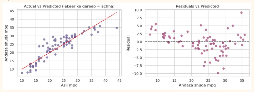
axes[0].set_title("Actual vs Predicted (near the line = good)")
axes[1].scatter(p, y_te - p, color="#A4457A", alpha=0.7)
axes[1].axhline(0, color="black", linestyle="--")
axes[1].set_xlabel("Predicted mpg")
axes[1].set_ylabel("Residual")
axes[1].set_title("Residuals vs Predicted")
plt.tight_layout()
plt.show()
OUTPUT (chart)
Step 8: How to do better? (one more attempt)
A slight pattern may be visible in the residual plot (the relationship is slightly curved). A common fix: take the log of the target. We compare both models using the same features and same test set , and measure RMSE on the original scale of mpg (converting the log model's predictions back to mpg with np.exp ).
train, test = train_test_split(cars, test_size=0.2, random_state=42)
feats = "weight + model_year + C(origin)"
lin = smf.ols("mpg ~ " + feats, data=train).fit()
log = smf.ols("np.log(mpg) ~ " + feats, data=train).fit()
def rmse(a, b):
    return float(np.sqrt(np.mean((a - b) ** 2)))
print("Linear model RMSE:", round(rmse(test["mpg"], lin.predict(test)), 2), "mpg")
print("Log model RMSE   :", round(rmse(test["mpg"], np.exp(log.predict(test))), 2), "mpg")
OUTPUT
Linear model RMSE: 3.33 mpg
Log model RMSE   : 2.75 mpg
Taking the log made the test RMSE lower , i.e. the log transform improved the prediction on this data. This shows that a model is not meant to be built once and left alone , but improved through experimentation.
Step 9: Report (writing up the result)
Be sure to write these parts in your project's README or report:
-
Goal: predicting mpg and the factors that affect it.
-
Data: 398 cars, 6 rows removed because of missing values (392 remain).
-
EDA findings: a strong negative relationship between weight and mpg; features are correlated with each other.
-
Models: Model 1 (weight only), Model 2 (several features), Model 3 (log mpg). For each: R<sup>2</sup> , test RMSE.
-
Most important effects: weight and model_year (with coefficients and p-values).
-
Limitations: old data (1970 to 1982), the relationship is not perfectly straight, features are correlated with each other.
-
Next step: comparison with Decision Tree/Random Forest in Module 4.
11.8 Hands-on
# Dataset: seaborn's 'tips'
tips = sns.load_dataset("tips")
print(tips[["total_bill", "tip", "size"]].corr().round(2))
OUTPUT
            total_bill   tip  size
total_bill        1.00  0.68  0.60
tip               0.68  1.00  0.49
size              0.60  0.49  1.00
-
Simple regression: tip ~ total_bill — fit this model. Report the slope and R<sup>2</sup> . Explain what the slope means in your own words.
-
Prediction: predict the tip for a bill of 40 dollars.
-
Multiple regression: tip ~ total_bill + size + C(smoker) + C(day) . Which features have a p-value below 0.05?
-
Residual plot: make residuals vs fitted. Is there any pattern? (Hint: the spread increases at larger bills)
-
Train/Test: do an 80/20 split and compute RMSE and R<sup>2</sup> .
-
Question to think about: is a higher bill the cause of a higher tip? What could a confounding variable be?
Challenge: Take the hours/marks dataset of Chapter 9, add an outlier (hours = 9, marks = 10) to it and rerun the regression. How much did the slope and R<sup>2</sup> change? This will give you a feel for the effect of outliers.
KEY TAKEAWAYS
-
Covariance gives direction; correlation (-1 to +1) gives strength too. Pearson is for straight-line relationships, Spearman for monotonic ones.
-
Correlation does not mean causation. The lesson of Anscombe: plot the data before modelling.
-
Simple linear regression: y = b0 + b1 x. Slope = the change in y for a 1-unit increase in x. Least squares minimizes the sum of squared residuals.
-
R-squared: how much of the spread in y the model explained. Avoid extrapolation.
-
The statsmodels report contains coef, std err, p-value, confidence interval, R-squared and the F-test.
-
In multiple regression a coefficient means: the effect of that x holding everything else equal. Check Adjusted R-squared and VIF.
-
Assumptions (LINE): Linearity, Independence, Normality of residuals, Equal variance. Check them with residual plots.
-
Metrics: MAE, MSE, RMSE, R-squared. Always evaluate on the test set (train/test split).