Chapter 41: Big Data
MODULE 7 | WEEK 41
Chapter 41: Big Data
Until now, the data you have seen has fit in your laptop's RAM (an Excel sheet, a CSV, a Pandas DataFrame). In the real world, companies like Daraz, Careem, Jazz, banks and YouTube generate terabytes (TB) and petabytes (PB) of data every day, which simply does not fit on one computer. In this chapter we will learn what Big Data is , why one computer is not enough, and how data is handled by splitting it across many computers ( HDFS, MapReduce, partitioning, batch and streaming ). We will first understand every idea by hand with small Python code , then in Chapter 42 do the same work much more easily in Apache Spark .
TOPIC CHECKLIST (tick them off as you go)
-
☐ What Big Data is and the 5 Vs (Volume, Velocity, Variety, Veracity, Value)
-
☐ The limit of one computer: scale up vs scale out
-
☐ Distributed storage: HDFS, blocks and replication
-
☐ MapReduce: Map, Shuffle, Reduce (word count)
-
☐ Row-based vs columnar formats (CSV, JSON, Parquet)
-
☐ Partitioning and data skew
-
☐ Batch vs streaming processing
-
☐ Big Data ecosystem: Hadoop, Hive, Kafka, Spark, NoSQL
-
☐ Data Lake vs Data Warehouse
41.1 What is Big Data?
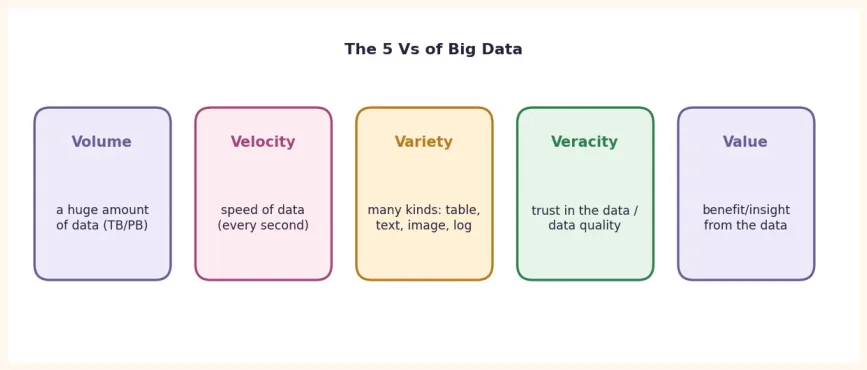
Big Data is data that is so big, fast-arriving or varied that a single computer and older tools (such as Excel or a single database) cannot handle it. Being "big" alone is not enough; data is judged by 5 characteristics , called the 5 Vs .
| V | Meaning | Example |
|---|---|---|
| Volume | The amount of data (GB to TB, PB) | A bank's transactions over many years; videos uploaded to YouTube every day |
| Velocity | How fast data is arriving | Thousands of UPI/Easypaisa transactions every second, Twitter/X posts |
| Variety | The many forms data comes in | Tables (structured), JSON/logs (semi-structured), images/video/audio (unstructured) |
| Veracity | How much the data can be trusted (wrong, incomplete, duplicate) | A faulty sensor reading, two records for one customer |
| Value | Getting something useful out of the data | Catching fraud, showing the right product, predicting traffic |
41.2 Why is one computer not enough? Scale up vs Scale out
When data grows, there are two ways to go:
| Scale Up (Vertical) | Scale Out (Horizontal) | |
|---|---|---|
| How | Make one computer more powerful (more RAM, CPU, bigger disk) | Join many ordinary computers together (a cluster) |
| Limit | Becomes expensive and then impossible after a point | Keep adding machines as needed |
| Failure | One machine fails = everything stops | One machine fails = the rest keep working |
| Example | From a 16 GB laptop to a 256 GB server | A cluster of 100 cheap machines |
| In Big Data | Rarely used | This is the standard(Hadoop, Spark) |
Let us work out a small calculation: how long would it take to read 1 TB of data from one disk reading at 200 MB/second , and if the same data were spread over 10 or 100 disks/machines ?
size_tb = 1
mb_per_sec = 200                      # speed of one disk
total_mb = size_tb * 1024 * 1024
for disks in [1, 10, 100]:
    sec = total_mb / (mb_per_sec * disks)
    print(f"{disks:>3} disk: {sec:>7.0f} seconds = {sec/60:>5.1f} minutes")
OUTPUT
  1 disk:    5243 seconds =  87.4 minutes
 10 disk:     524 seconds =   8.7 minutes
100 disk:      52 seconds =   0.9 minutes
On one machine, reading 1 TB takes about 87 minutes , whereas if 100 machines read together it takes less than 1 minute . This parallel (simultaneous) work is the heart of Big Data.
41.3 Distributed Storage: HDFS
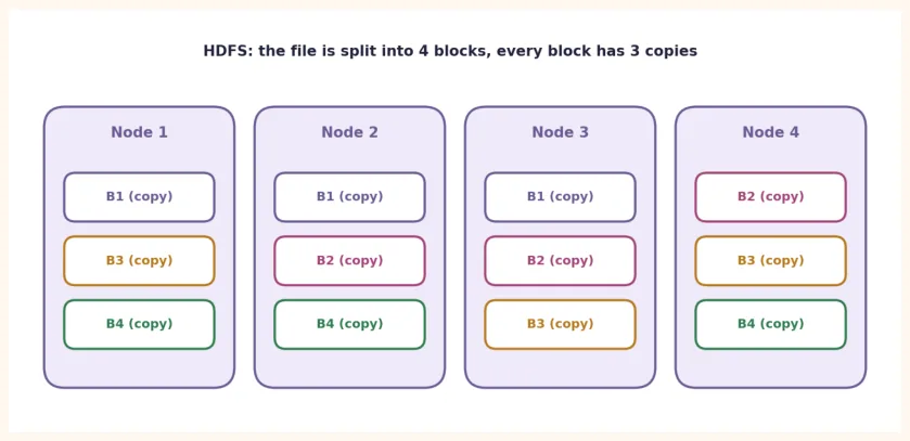
HDFS (Hadoop Distributed File System) is a file system that splits one big file into pieces (blocks) and stores them on many machines . It has three basic ideas:
-
Blocks: splitting a file into equal pieces (typically 128 MB per block).
-
Replication: 3 copies of every block on different machines (by default). If one machine fails, no data is lost.
-
NameNode and DataNodes: NameNode keeps the "index" (which block is on which machine), DataNodes hold the actual blocks.
OUTPUT
Number of blocks: 4
B1 -> ['N2', 'N5', 'N4']
B2 -> ['N5', 'N4', 'N3']
B3 -> ['N5', 'N1', 'N3']
B4 -> ['N1', 'N4', 'N2']
N2 failed: True
Two machines failing together: file safe in 10/10 cases
Because every block has 3 copies , even if any 2 machines fail at the same time, at least one copy of every block survives. This is called fault tolerance (the ability to survive failures).
NOTE
Why is a block big? Small blocks mean a huge amount of index data (metadata) and a lot of small reads. A big block like 128 MB reduces the effort of disk seeking (searching) . Nowadays people also use cloud object storage (S3, Azure Blob) alongside HDFS, which we will cover in Chapter 43.
41.4 MapReduce: a way to do work in parts
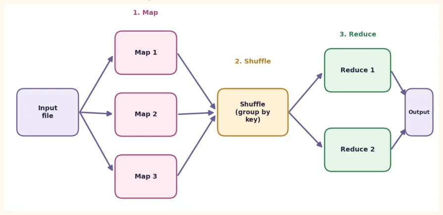
MapReduce is a programming model that splits any big job into 3 steps :
-
Map: each machine works on its own part of the data and produces (key, value) pairs.
-
Shuffle: pairs with the same key are gathered in one place.
-
Reduce: all the values of each key are combined (sum, count, max) into one answer.
Word Count: the "Hello World" of MapReduce
from collections import defaultdict
lines = ["spark is fast",
"hadoop is old spark is new",
"big data is"]
# 1) MAP:
for every word make (word, 1)
mapped = []
for line in lines:
    for word in line.split():
        mapped.append((word, 1))
        print("MAP    :", mapped[:4], "...")
        # 2) SHUFFLE: same keys in one place
        groups = defaultdict(list)
        for key, value in mapped:
            groups[key].append(value)
            print("SHUFFLE:")
            for key, vals in groups.items():
                print("   ", key, vals)
                # 3) REDUCE: sum of the values of each key
                result = {key: sum(vals) for key, vals in groups.items()}
                print("REDUCE :")
                for key, total in result.items():
                    print("   ", key, total)
OUTPUT
MAP    : [('spark', 1), ('is', 1), ('fast', 1), ('hadoop', 1)] ...
SHUFFLE:
    spark [1, 1]
    is [1, 1, 1, 1]
    fast [1]
    hadoop [1]
    old [1]
    new [1]
    big [1]
    data [1]
REDUCE :
    spark 2
    is 4
    fast 1
    hadoop 1
    old 1
    new 1
    big 1
    data 1
In real Hadoop, Map and Reduce run on different machines and the intermediate data is written to disk , which is why MapReduce is slow . To fix exactly this weakness, Spark arrived (Chapter 42).
41.5 Data formats: Row-based vs Columnar
In Big Data, the form in which data is stored matters a great deal. A file can be stored in two ways:
-
Row-based (CSV, JSON): all the columns of one row together. Good for finding or writing a single record.
-
Columnar (Parquet, ORC): all the values of one column together. Very fast and compact for analytics (the sum/average of just a few columns).
For example, from 1000 rows we only need the total of the amount column. Let us see how many values have to be touched in each approach:
# row-store: each row = (id, city, amount, qty)
rows = [(i, "Karachi", 100 + i, 5) for i in range(1000)]
columns = {                                                # column-store
    "id":     [r[0] for r in rows],
    "city":   [r[1] for r in rows],
    "amount": [r[2] for r in rows],
    "qty":    [r[3] for r in rows],
}
# Row-store: every row has to be read in full (4 values)
touched_row = sum(len(r) for r in rows)
total_row = sum(r[2] for r in rows)
# Column-store: only the 'amount' column
touched_col = len(columns["amount"])
total_col = sum(columns["amount"])
print("Row-store   :", touched_row, "values touched, total =", total_row)
print("Column-store:", touched_col, "values touched, total =", total_col)
OUTPUT
Row-store   : 4000 values touched, total = 599500
Column-store: 1000 values touched, total = 599500
| Format | Type | Key feature | When to use |
|---|---|---|---|
| CSV | Row, text | Simple, opens everywhere; large and slow | Small data, sharing |
| JSON | Row, text | Can hold nested data; large | APIs, logs |
| Parquet | Columnar, binary | Compressed, carries its schema, reads only the columns it needs | The standard for Big Data analytics |
| ORC | Columnar, binary | Similar to Parquet, common in Hive | Hive/Hadoop ecosystem |
41.6 Partitioning and Data Skew
Splitting data across machines is called partitioning . The most common method is hash partitioning : the hash of each record's key is computed, and hash % partitions decides which partition it goes to. In good partitioning every partition gets roughly equal work .
def h(key):
    # simple deterministic hash
    v = 0
    for ch in str(key):
        v = (v * 31 + ord(ch)) % 1000003
    return v
def partition_sizes(keys, n=4):
    sizes = [0] * n
    for k in keys:
        sizes[h(k) % n] += 1
    return sizes
balanced = [f"cust{i}" for i in range(1000)]
skewed   = ["cust_hot"] * 600 + [f"cust{i}" for i in range(400)]
print("Balanced:", partition_sizes(balanced))
print("Skewed  :", partition_sizes(skewed))
OUTPUT
Balanced: [251, 249, 249, 251]
Skewed  : [102, 700, 98, 100]
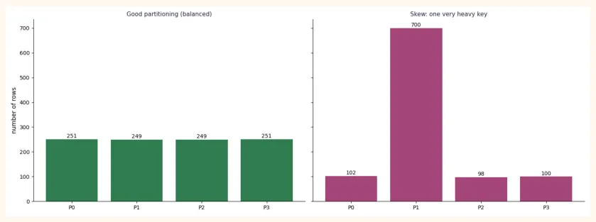
In the second case one key ( cust_hot ) has 600 records, so all the load landed on one partition while the other machines sit idle . This is Data Skew : the whole job becomes as slow as its slowest partition. The fixes: choose a better key, use salting (add a random word to the key), or handle the skewed key separately.
41.7 Batch vs Streaming
| Batch | Streaming | |
|---|---|---|
| Data | Accumulated, a whole file/table | Arriving continuously (event by event) |
| When it runs | At fixed times (every night, every hour) | All the time, within a few seconds |
| Latency | Minutes to hours | Milliseconds to seconds |
| Example | A report of the whole day's sales at night | An instant card-fraud alert, live traffic |
| Tools | Hadoop MapReduce, Spark | Kafka, Spark Structured Streaming, Flink |
In streaming, data is usually counted by splitting it into time windows . Below is a small example of 5-second
tumbling windows :
# each event = (second, user)
events = [(1, "A"), (3, "B"), (4, "A"), (7, "A"), (8, "B"), (11, "A")]
window = 5
counts = {}
for t, user in events:
    start = (t // window) * window
    counts[start] = counts.get(start, 0) + 1
for start in sorted(counts):
    print(f"[{start:>2}s to {start + window:>2}s): {counts[start]} events")
OUTPUT
[ 0s to  5s): 3 events
[ 5s to 10s): 2 events
[10s to 15s): 1 events
41.8 The Big Data Ecosystem at a Glance
| Task | Tool | In one line |
|---|---|---|
| Storage | HDFS, S3, Azure Blob/ADLS | Keeping big data on many machines/in the cloud |
| Task | Tool | In one line |
|---|---|---|
| Batch processing | Hadoop MapReduce,Apache Spark | Calculations on big data; Spark is faster |
| SQL on big data | Hive, Spark SQL, Presto/Trino, Athena | Running SQL on big data |
| Messaging / ingest | Apache Kafka, Kinesis, Event Hubs | Bringing live data into a pipeline |
| Stream processing | Spark Structured Streaming,Flink | Calculations on live data |
| NoSQL database | MongoDB, Cassandra, HBase, DynamoDB | Very fast writes/reads, flexible schema |
| Orchestration | Airflow, Azure Data Factory | Sequencing and scheduling of jobs |
41.9 Data Lake vs Data Warehouse
| Data Warehouse | Data Lake | |
|---|---|---|
| Form of data | Clean, structured tables | Raw data of every kind (CSV, JSON, images, logs) |
| Schema | Defined first (schema-on-write) | Defined at read time (schema-on-read) |
| Cost | Higher | Lower (cheap object storage) |
| Used for | BI dashboards, reports | Data science, ML, raw archive |
| Example | Redshift, Synapse, BigQuery, Snowflake | S3, Azure Data Lake Storage |
Today's trend is the Lakehouse : warehouse-like tables and SQL on the cheap storage of a Data Lake (Delta Lake, Apache Iceberg). This will also be touched on in Chapters 40-41.
41.10 Common Mistakes and Hands-on
Hands-on
- Scale: In 38.2, set
size_tb = 10
and
disks = 500
and calculate; how much time does it take?
- HDFS: Set
file_mb = 1000
and
replicas = 2
. Is the file still safe when any 2 machines fail together? Why or why not?
-
MapReduce: Put your own 5 favourite sentences in
linesand compute the word count; which word appears most? -
Columnar: Now compute the average of
qtyin both row-store and column-store and see how many values were touched. -
Skew: In the
skewedlist, change the count ofcust_hotfrom 600 to 100 and look at the partition sizes. -
Streaming: Set
window = 3
and look at the result.
KEY TAKEAWAYS
-
Big Data = very large, fast or varied data that one computer cannot handle: the 5 Vs (Volume, Velocity, Variety, Veracity, Value).
-
Scale out (many cheap machines) is the standard solution for Big Data; scale up has a limit.
-
HDFS: a file is broken into blocks and every block has 3 copies ( fault tolerance ).
-
MapReduce: Map (make key, value) -> Shuffle (gather by key) -> Reduce (sum/count).
-
For analytics, columnar formats (Parquet) are faster and smaller than row-based formats (CSV).
-
Partitioning splits the work; data skew puts the load on one machine.
-
Batch = accumulated data, Streaming = continuous data; Data Lake (raw, cheap) vs Warehouse (clean, structured).