Chapter 42: Apache Spark
MODULE 7 | WEEK 42
Chapter 42: Apache Spark
In Chapter 41 we saw that work on big data is done by splitting it across many machines , and the old MapReduce writes data to disk after every step, which makes it slow. Apache Spark does the same work in memory (RAM) and offers an easy API in Python, SQL, Scala and Java. Most Big Data companies in the world use Spark today. In this chapter we will learn PySpark (the Python side of Spark): RDD, DataFrame, Spark SQL, lazy evaluation, joins, window functions, performance and Parquet , and finally a short look at MLlib .
TOPIC CHECKLIST (tick them off as you go)
-
☐ What Spark is and why it is faster than MapReduce
-
☐ Spark's structure: Driver, Executors, Cluster Manager
-
☐ SparkSession and setup in Colab
-
☐ RDD: parallelize, map, filter, reduceByKey
-
☐ DataFrame: schema, select, filter, withColumn, groupBy, agg
-
☐ Spark SQL (temporary view)
-
☐ Lazy evaluation, Transformations vs Actions, DAG
-
☐ Joins and Window functions
-
☐ Performance: partitions, cache, broadcast join, Parquet
-
☐ MLlib: a small Pipeline example
-
☐ Pandas vs Spark: which to use when
42.1 What is Spark and why is it fast?
Apache Spark is an open-source distributed computing engine that does fast, parallel work on big data. It has three big advantages:
-
In-memory processing: intermediate results stay in RAM instead of being written to disk at every step. That is why it is many times faster than MapReduce for iterative work (machine learning).
-
One engine, many jobs: batch, SQL, streaming, machine learning (MLlib), graphs.
-
Easy API: Python (PySpark), SQL, Scala, Java, R.
| Component | Job |
|---|---|
| Spark Core (RDD) | Foundation: splitting work, memory, fault tolerance |
| Spark SQL / DataFrame | Table-like data and SQL; the most widely used |
| Structured Streaming | The same DataFrame code on live data |
| MLlib | Distributed machine learning |
| GraphX | Graph analysis (Scala/Java) |
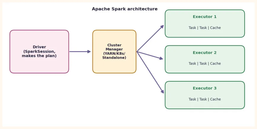
| Component | What it does |
|---|---|
| Driver | Your program runs here.SparkSessionlives here. It makes theplanfor the work and sends out tasks. |
| Cluster Manager | Hands out the machines' resources (CPU/RAM) (Standalone, YARN, Kubernetes). |
| Executor | Processes on worker machines thatrun tasksandcachedata. |
| Task / Partition | One piece of data and the small job done on it. One partition = one task. |
42.2 Setup: SparkSession and the dataset
In Colab, install it in one cell and create a SparkSession . local[*] means use all the cores of your one machine (enough for learning; on a cluster this changes).
!pip install pyspark
from pyspark.sql import SparkSession
spark = (SparkSession.builder
         .appName("Module8")
         .master("local[*]")
         .getOrCreate())
print(spark.version)
OUTPUT (sample; your version may differ) 4.0.0
Now we create 5000 rows of sales data for this chapter and Chapter 44. This code runs anywhere (Python only), and because of seed 42 it produces exactly the same data every time:
import random, csv
from datetime import date, timedelta
random.seed(42)
cities = ["Karachi", "Lahore", "Islamabad", "Quetta", "Peshawar"]
price_range = {"Mobile": (25000, 90000), "Laptop": (60000, 250000), "Headphones": (2000, 15000), "Watch": (5000, 40000)}
start = date(2025, 1, 1)
with open("sales.csv", "w", newline="") as f:
    w = csv.writer(f)
    w.writerow(["order_id", "order_date", "city", "category", "qty", "unit_price", "customer_id"])
    for i in range(1, 5001):
        cat = random.choice(list(price_range))
        lo, hi = price_range[cat]
        d = start + timedelta(days=random.randint(0, 364))
        w.writerow([i, d.isoformat(), random.choice(cities), cat, random.randint(1, 4), random.randrange(lo, hi, 500), random.randint(1, 800)])
        print("sales.csv is ready")
OUTPUT sales.csv is ready
In Colab, run the file and the code above in the same place ( sales.csv will appear in the Files panel). The first 3 rows:
OUTPUT (sample; the first 3 rows of sales.csv)
+--------+----------+---------+--------+---+----------+-----------+
|order_id|order_date|     city|category|qty|unit_price|customer_id|
+--------+----------+---------+--------+---+----------+-----------+
|       1|2025-01-13|Islamabad|  Mobile|  2|     53500|        143|
|       2|2025-12-13| Peshawar|  Mobile|  1|     79000|         33|
|       3|2025-02-17|   Lahore|  Mobile|  2|     89500|        617|
+--------+----------+---------+--------+---+----------+-----------+
42.3 RDD: the foundation of Spark
RDD (Resilient Distributed Dataset) is Spark's oldest and most basic data structure: a list that is spread across many machines (partitions) . Resilient means: if a machine fails, Spark rebuilds that part from the remembered plan (lineage) . Nowadays we mostly use DataFrame , but understanding RDD is understanding Spark.
sc = spark.sparkContext
lines = sc.parallelize([
"spark is fast",
"hadoop is old spark is new",
"big data is",
])
counts = (lines
.flatMap(lambda line: line.split())      # each sentence -> words
.map(lambda w: (w, 1))                   # (word, 1)
.reduceByKey(lambda a, b: a + b))        # sum by key
print(counts.sortBy(lambda kv: (-kv[1], kv[0])).collect())
OUTPUT (sample) [('is', 4), ('spark', 2), ('big', 1), ('data', 1), ('fast', 1), ('hadoop', 1), ('new', 1), ('old', 1)]
This is the same Word Count we did by hand in Chapter 41; now flatMap / map is the Map and reduceByKey is the Shuffle + Reduce . The only difference is that Spark spreads this work across many machines by itself.
| Operation | Type | What it does |
|---|---|---|
map(f) | Transformation | Applies f to every element |
filter(f) | Transformation | Keeps only the elements for which f is True |
flatMap(f) | Transformation | Produces 0 or more elements from each element |
reduceByKey(f) | Transformation (shuffle) | Combines the values of the same key |
collect() | Action | Brings all the data to the driver (dangerous on big data) |
count(),take(n) | Action | Count / the first n elements |
42.4 DataFrame: table-like distributed data
DataFrame looks like a Pandas DataFrame (rows and named columns), but underneath it is spread across many machines and Spark's optimizer (Catalyst) makes the work on it faster. That is why DataFrame/SQL is the first choice in production.
Reading a CSV (write the schema yourself)
inferSchema=True reads the data twice (slow), and may also get a type wrong. For big data it is better to write the schema yourself :
from pyspark.sql.types import (
    StructType,
    StructField,
    IntegerType,
    StringType,
    DateType,
)

schema = StructType([
    StructField("order_id", IntegerType(), True),
    StructField("order_date", DateType(), True),
    StructField("city", StringType(), True),
    StructField("category", StringType(), True),
    StructField("qty", IntegerType(), True),
    StructField("unit_price", IntegerType(), True),
    StructField("customer_id", IntegerType(), True),
])
sales = spark.read.csv("sales.csv", header=True, schema=schema)
sales.printSchema()
print(sales.count())
OUTPUT (sample)
root
 |-- order_id: integer (nullable = true)
 |-- order_date: date (nullable = true)
 |-- city: string (nullable = true)
 |-- category: string (nullable = true)
 |-- qty: integer (nullable = true)
 |-- unit_price: integer (nullable = true)
 |-- customer_id: integer (nullable = true)
5000
select, filter, withColumn
from pyspark.sql import functions as F
big = (sales
.withColumn("revenue", F.col("qty") * F.col("unit_price"))   # new column
.filter(F.col("city") == "Karachi")                          # Karachi only
.select("order_id", "category", "qty", "unit_price", "revenue"))
big.show(3)
OUTPUT (sample)
+--------+--------+---+----------+-------+
|order_id|category|qty|unit_price|revenue|
+--------+--------+---+----------+-------+
|       8|   Watch|  4|     10000|  40000|
|      15|  Mobile|  3|     76000| 228000|
|      20|  Mobile|  2|     45000|  90000|
+--------+--------+---+----------+-------+
groupBy and agg
sales = sales.withColumn("revenue", F.col("qty") * F.col("unit_price"))
by_cat = (sales.groupBy("category")
.agg(F.count("*").alias("orders"),
F.sum("revenue").alias("total_revenue"),
F.round(F.avg("revenue"), 2).alias("avg_order"))
.orderBy(F.desc("total_revenue")))
by_cat.show()
OUTPUT (sample)
+----------+------+-------------+---------+
|  category|orders|total_revenue|avg_order|
+----------+------+-------------+---------+
|    Laptop|  1260|    494225000|392242.06|
|    Mobile|  1263|    183377500| 145192.0|
|     Watch|  1246|     67262500| 53982.74|
|Headphones|  1231|     25482000| 20700.24|
+----------+------+-------------+---------+
Verification: let us do the same calculation with Pandas (this OUTPUT is real). The results of both should be the same:
import pandas as pd
pdf = pd.read_csv("sales.csv")
pdf["revenue"] = pdf["qty"] * pdf["unit_price"]
res = (pdf.groupby("category")["revenue"]
.agg(orders="count", total_revenue="sum", avg_order="mean")
.round(2)
.sort_values("total_revenue", ascending=False))
print(res)
OUTPUT
            orders  total_revenue  avg_order
category
Laptop        1260      494225000  392242.06
Mobile        1263      183377500  145192.00
Watch         1246       67262500   53982.74
Headphones    1231       25482000   20700.24
By month and by city
monthly = (sales
.groupBy(F.month("order_date").alias("month"))
.agg(F.sum("revenue").alias("revenue"))
.orderBy("month"))
monthly.show(4)
city_rev = (sales.groupBy("city")
.agg(F.sum("revenue").alias("revenue"))
.orderBy(F.desc("revenue")))
city_rev.show()
OUTPUT (sample)
+-----+--------+
|month| revenue|
+-----+--------+
|    1|69752000|
|    2|59793500|
|    3|60314000|
|    4|66487000|
+-----+--------+
+---------+---------+
|     city|  revenue|
+---------+---------+
|   Lahore|171351000|
| Peshawar|159378000|
|Islamabad|151400500|
|  Karachi|150230500|
|   Quetta|137987000|
+---------+---------+
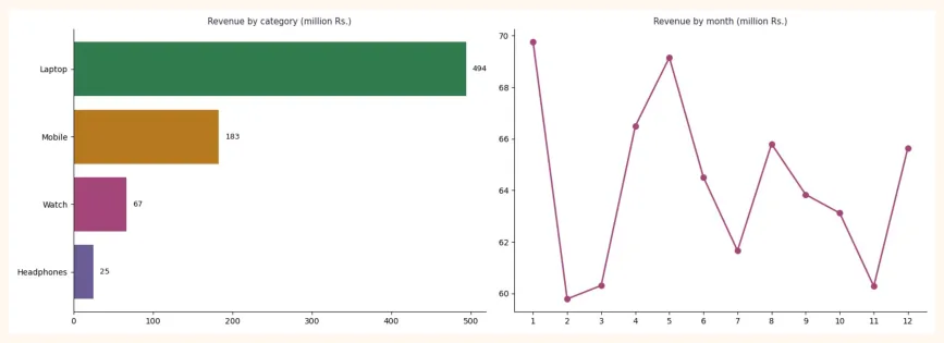
You can turn a small result into Pandas ( toPandas() ) and draw a chart. Careful: toPandas() brings all the data into the driver's memory, so run it only on small aggregated results , not on the whole big dataset.
import matplotlib.pyplot as plt
pdf_cat = by_cat.toPandas()                       # small result (4 rows)
pdf_mon = monthly.toPandas()
# then a bar chart and a line chart
with matplotlib (as in Module 2)
42.5 Spark SQL
If you know SQL, you can turn a DataFrame into a temporary view and write SQL directly. The DataFrame and SQL run on the same engine , so the speed is the same.
sales.createOrReplaceTempView("sales")
top = spark.sql("""
    SELECT customer_id,
           COUNT(*)      AS orders,
           SUM(revenue)  AS spent
    FROM sales
    GROUP BY customer_id
    ORDER BY spent DESC
    LIMIT 3
""")
top.show()
OUTPUT (sample)
+-----------+------+-------+
|customer_id|orders|  spent|
+-----------+------+-------+
|        615|    11|3319500|
|        397|     9|3078000|
|         69|    14|3035500|
+-----------+------+-------+
42.6 Lazy Evaluation, Transformations and Actions
The most important thing about Spark: when you write filter , select , withColumn , groupBy and other transformations , Spark does not run anything ; it only remembers a plan (DAG) . The work starts only when you run an action ( show , count , collect , write ).
| Transformations (lazy) | Actions (work starts) |
|---|---|
select,filter/where,withColumn | show(),count() |
groupBy().agg(),join,orderBy | collect(),take(n),first() |
repartition,distinct,drop | write.parquet(...),toPandas() |
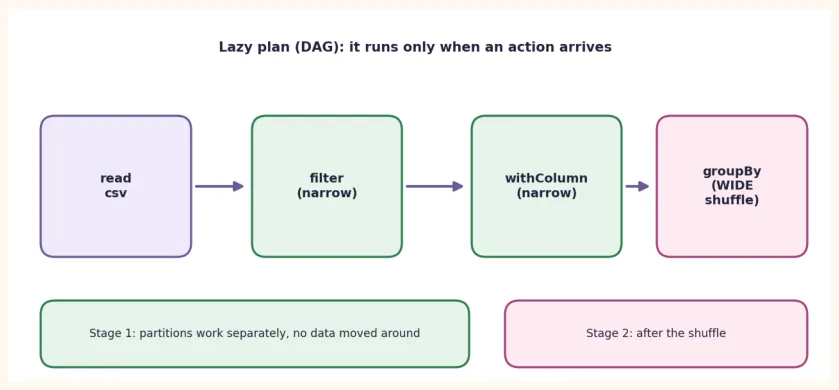
Narrow vs Wide transformations:
-
Narrow (
filter,select,withColumn): each partition works on its own , and no data has to be sent between machines . Cheap and fast. -
Wide (
groupBy,join,orderBy,distinct): data has to be sent between partitions (shuffle) , which is expensive because of the network and disk. Spark breaks the plan into stages : a new stage at every wide transformation.
(sales.filter(F.col("qty") > 1)
      .groupBy("city")
      .agg(F.count("*").alias("n"))
      .explain())
OUTPUT (sample; the detailed form of the plan varies with the version)
== Physical Plan == AdaptiveSparkPlan
isFinalPlan=false +- HashAggregate(keys=[city#2], functions=[count(1)]) +- Exchange hashpartitioning(city#2, 200)     <-- this is the SHUFFLE +- HashAggregate(keys=[city#2], functions=[partial_count(1)]) +- Filter (isnotnull(qty#4) AND (qty#4 > 1)) +- FileScan csv [city#2,qty#4] ...
explain() If you see Exchange in the output, understand that a shuffle is happening there. Improving performance often means reducing shuffles.
42.7 Joins and Window Functions
Join
regions = spark.createDataFrame(
[("Karachi", "Sindh"), ("Lahore", "Punjab"), ("Islamabad", "Capital"),
("Quetta", "Balochistan"), ("Peshawar", "KP")],
["city", "region"])
joined = sales.join(regions, on="city", how="left")
(joined.groupBy("region")
.agg(F.sum("revenue").alias("revenue"))
.orderBy(F.desc("revenue"))
.show())
OUTPUT (sample)
+-----------+---------+
|     region|  revenue|
+-----------+---------+
|     Punjab|171351000|
|         KP|159378000|
|    Capital|151400500|
|      Sindh|150230500|
|Balochistan|137987000|
+-----------+---------+
| Join type | Result |
|---|---|
inner | Only the rows whose key is in both tables |
left | All rows of the left table; null if there is no match on the right |
right | All rows of the right table |
outer | All rows of both |
left_semi/left_anti | The rows of the left whose keyis/is notin the right (the right's columns do not come through) |
Window function: ranking within each group
groupBy reduces the rows. A Window function keeps the rows but does calculations (rank, running total) within a group . For example: the city with the highest revenue in each category :
from pyspark.sql.window import Window
cc = (sales.groupBy("category", "city")
.agg(F.sum("revenue").alias("revenue")))
w = Window.partitionBy("category").orderBy(F.desc("revenue"))
(cc.withColumn("rank", F.row_number().over(w))
.filter(F.col("rank") == 1)
.orderBy("category")
.show())
OUTPUT (sample)
+----------+------+---------+----+
|  category|  city|  revenue|rank|
+----------+------+---------+----+
|Headphones|Quetta|  5437000|   1|
|    Laptop|Lahore|110832500|   1|
|    Mobile|Lahore| 40554000|   1|
|     Watch|Lahore| 14556500|   1|
+----------+------+---------+----+
42.8 Performance: partitions, cache and Parquet
| Technique | Why and how |
|---|---|
| Filter early, select early | Reduce rows and columns before the heavy work (join/groupBy). |
| Built-in functions (F.*) | Many times faster than a Python UDF, because Spark can optimize them. |
| Store in Parquet | Columnar + compressed; reads only the columns it needs. |
| cache() / persist() | Keep a DataFrame that is used again and again in memory. |
| repartition(n) / coalesce(n) | repartitionsplits evenly with a shuffle;coalesce reducespartitions without ashuffle. |
| Broadcast join | Avoid a shuffle when joining with a small table. |
| Avoid collect() | Bringing all the data to the driver can use up its memory. |
clean = sales.filter(F.col("qty") > 0).cache()      # keep in memory
print(clean.count())                                # first action: fills the cache
print(clean.count())                                # second:
from the cache, fast
print(clean.rdd.getNumPartitions())
print(clean.repartition(8).rdd.getNumPartitions())
print(clean.coalesce(2).rdd.getNumPartitions())
clean.unpersist()                                   # when the work is done, empty the cache
OUTPUT (sample; a small file often has few partitions) 5000 5000 1 8 1
Note: coalesce(2) can only reduce partitions; if there is already 1, it stays at 1.
Writing and reading Parquet
(sales.write
      .mode("overwrite")
      .partitionBy("category")          # a separate folder per category
      .parquet("sales_parquet"))
fast = spark.read.parquet("sales_parquet")
# only the Laptop folder is read
fast.filter(F.col("category") == "Laptop").count()
OUTPUT (sample: the folder structure and the count) sales_parquet/ _SUCCESS category=Headphones/part-....snappy.parquet category=Laptop/part-....snappy.parquet category=Mobile/part-....snappy.parquet category=Watch/part-....snappy.parquet
1260
partitionBy("category") splits the data into folders , and when you filter on category, Spark reads only the necessary folder ( partition pruning ). Use partitionBy only on a column with few unique values (category, yearmonth); on a column like customer_id you would create thousands of tiny folders.
42.9 A short look at MLlib: groups of customers
MLlib is Spark's machine learning library. Its Pipeline is like scikit-learn's, but the data stays distributed. Below is an example of splitting customers into 3 groups by their spending and orders ( KMeans , recall Module 4 Chapter 16).
from pyspark.ml.feature import VectorAssembler, StandardScaler
from pyspark.ml.clustering import KMeans
from pyspark.ml import Pipeline
cust = (sales.groupBy("customer_id")
.agg(F.count("*").alias("orders"),
F.sum("revenue").alias("spent")))
assembler = VectorAssembler(inputCols=["orders", "spent"], outputCol="raw")
scaler    = StandardScaler(inputCol="raw", outputCol="features")
kmeans    = KMeans(k=3, seed=42, featuresCol="features")
model = Pipeline(stages=[assembler, scaler, kmeans]).fit(cust)
result = model.transform(cust)
result.groupBy("prediction").count().orderBy("prediction").show()
OUTPUT (sample; the group sizes may differ in your run) +----------+-----+ |prediction|count| +----------+-----+ | 0| ...| | 1| ...| | 2| ...| +----------+-----+
This is only a glimpse : the real benefit of MLlib comes when the data is so big that scikit-learn cannot run on one machine. For small data, scikit-learn is better and has more features.
42.10 Pandas vs Spark: which to use when?
| Pandas | Spark (PySpark) | |
|---|---|---|
| Data size | Up to one machine's RAM (typically GBs) | GB to PB, on a cluster |
| Speed (small data) | Fast | Start-up overhead, slow on small data |
| Lazy? | No, runs immediately | Yes, runs on an action |
| Data | In memory, mutable | Distributed, immutable (every step makes a new DataFrame) |
| Learning curve | Easy | A bit more (shuffle, partitions, plan) |
| When | EDA, small projects | Big logs, pipelines, production ETL |
42.11 Common Mistakes and Hands-on
Hands-on
-
RDD: in the word count, put in your own 5 sentences and keep only the words that occur 2 or more times (
filter). -
DataFrame: Count the rows where
qty >= 3
and
city == "Lahore"
.
- New column: Create
revenue_lakh = revenue / 100000
and apply round(..., 2) .
-
groupBy: for each
cityandcategorypair, compute the average qty and show the top 5. -
SQL: write the
by_catcalculation above in SQL and match the result. -
Window: find the best-selling category of each month (
row_number). -
Performance: In the output of
explain(), look forExchange. Does it appear in a filter-only query withoutgroupBy? -
Parquet: Write with
partitionBy("city")and count the folders.
KEY TAKEAWAYS
-
Spark = an in-memory distributed engine: the Driver makes the plan, Executors run the tasks, the Cluster Manager allocates resources.
-
RDD is the foundation; DataFrame + Spark SQL are the everyday tools (fast thanks to the optimizer).
-
Lazy evaluation: transformations only build a plan (DAG); work happens on an action .
-
Narrow transformations are cheap; wide ones (groupBy, join, orderBy) shuffle and are expensive.
-
Write the schema yourself , filter/select early, use built-in functions, Parquet and cache .
-
For a join with a small table use a broadcast join ; use
collect()andtoPandas()only on small results. -
For small data use Pandas , for big data use Spark .