Chapter 21: Neural Network Fundamentals and Backpropagation
MODULE 5 | WEEK 21
Chapter 21: Neural Network Fundamentals and Backpropagation
Now we step into the world of Deep Learning . In Module 4 you saw that a model learns from data; now we will see how a neural network , inspired by the human brain, learns: what a neuron, layer, activation and loss are, and most importantly, how a network learns from its own mistakes through backpropagation . First we will build everything by hand in NumPy so that the magic makes sense, and then we will do the same thing in TensorFlow/Keras in just a few lines.
21.1 What are Deep Learning and a Neural Network?
A Neural Network is a model built by joining many small neurons (units that do a little calculation) into layers . When there are a lot of layers ( deep ), we call it Deep Learning . Remember the umbrella from Chapter 1: AI > Machine Learning > Deep Learning .
21.2 One neuron: the smallest unit
A neuron does these 3 things: (1) multiplies each input by its own weight , (2) adds everything up and adds a bias , (3) passes the result through an activation function .
z = w1*x1 + w2*x2 + ... + wn*xn + b      (weighted sum)
a = activation(z)                           (output of the neuron)
21.3 Activation Functions
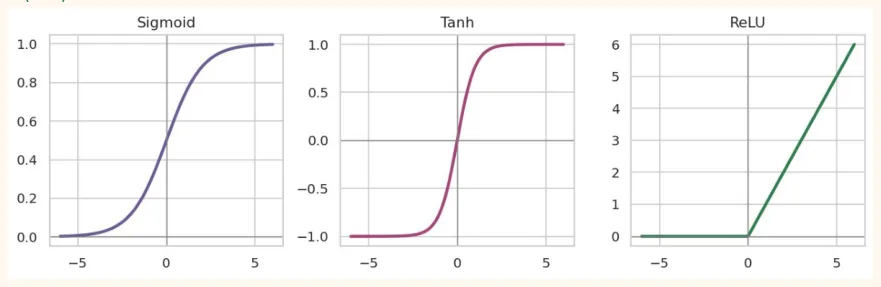
Without an activation, no matter how many layers you stack, the whole network turns into just one straight line (linear) . The activation function brings non-linearity (bendiness) into the network, which lets it learn complex patterns.
| Activation | Formula (short) | Output range | Where it is used |
|---|---|---|---|
| Sigmoid | 1 / (1 + e^-z) | 0 to 1 | Last layer of binary classification |
| Tanh | (e^z - e^-z) / (e^z + e^-z) | -1 to 1 | Older hidden layers, inside RNNs |
| ReLU | max(0, z) | 0 to infinity | Default for hidden layers |
| Softmax | e^zi / sum(e^zj) | 0 to 1 (sum = 1) | Last layer of multiclass classification |
import numpy as np
import matplotlib.pyplot as plt
z = np.linspace(-6, 6, 200)
funcs = {
"Sigmoid": 1 / (1 + np.exp(-z)),
"Tanh": np.tanh(z),
"ReLU": np.maximum(0, z),
}
colors = ["#6B5B95", "#A4457A", "#2F7D4F"]
fig, axes = plt.subplots(1, 3, figsize=(10, 3.2))
for ax, (name, y), c in zip(axes, funcs.items(), colors):
    ax.plot(z, y, color=c, lw=2.5)
    ax.axhline(0, color="gray", lw=0.8)
    ax.axvline(0, color="gray", lw=0.8)
    ax.set_title(name)
    plt.tight_layout()
    plt.show()
OUTPUT (chart)
Softmax turns a list of numbers (scores) into probabilities whose sum is always 1:
def softmax(scores):
    e = np.exp(scores - np.max(scores))   # subtract the max for stability
    return e / e.sum()
scores = np.array([2.0, 1.0, 0.1])         # raw scores
for 3 classes
p = softmax(scores)
print("Probabilities:", p.round(3))
print("Sum:", p.sum().round(3))
print("Predicted class:", p.argmax())
OUTPUT
Probabilities:
[0.659 0.242 0.099] Sum:
1.0 Predicted class:
0
21.4 Layers and Forward Propagation
Neurons in a network sit in layers : the Input layer (takes the data), one or more Hidden layers (the thinking inside), and the Output layer (the result). Data flows from the input towards the output, and this is called Forward Propagation . The calculation for a whole layer is done with matrix multiplication .
Layer calculation:   A = activation( X @ W + b )
X : (samples, input_features)
W : (input_features, neurons)
b : (neurons,)
A : (samples, neurons)
np.random.seed(0)
X = np.random.randn(5, 4)          # 5 samples, 4 features
W1 = np.random.randn(4, 3) * 0.5   # hidden layer: 3 neurons
b1 = np.zeros(3)
W2 = np.random.randn(3, 1) * 0.5   # output layer: 1 neuron
b2 = np.zeros(1)
relu = lambda z: np.maximum(0, z)
sigmoid = lambda z: 1 / (1 + np.exp(-z))
H = relu(X @ W1 + b1)              # output of the hidden layer
out = sigmoid(H @ W2 + b2)         # final probability
print("X shape  :", X.shape)
print("H shape  :", H.shape)
print("out shape:", out.shape)
print("Probabilities:", out.ravel().round(3))
print("Parameters:", W1.size + b1.size + W2.size + b2.size)
OUTPUT X shape : (5, 4) H shape : (5, 3) out shape: (5, 1) Probabilities: [0.2 0.405 0.269 0.382 0.423] Parameters: 19
21.5 Loss Function: a measure of the network's error
Loss tells us how far the network's prediction is from the truth. The goal of training is to make this loss as small as possible (remember the cost function from Chapter 13).
| Problem | Loss | Last layer |
|---|---|---|
| Regression | MSE (Mean Squared Error) | 1 neuron, no activation |
| Binary classification | Binary Cross-Entropy | 1 neuron, sigmoid |
| Multiclass (labels 0,1,2...) | Sparse Categorical Cross-Entropy | N neurons, softmax |
| Multiclass (one-hot labels) | Categorical Cross-Entropy | N neurons, softmax |
y_true = np.array([1, 0, 1, 1])
y_pred = np.array([0.9, 0.2, 0.6, 0.3])   # the network's probabilities
mse = np.mean((y_true - y_pred) ** 2)
bce = -np.mean(y_true * np.log(y_pred) + (1 - y_true) * np.log(1 - y_pred))
print("MSE:", round(mse, 4))
print("Binary Cross-Entropy:", round(bce, 4))
# If the network is very confident but wrong, cross-entropy shoots up
print("Correct and confident (0.99):", round(-np.log(0.99), 3))
print("Wrong and confident (0.01):", round(-np.log(0.01), 3))
OUTPUT MSE: 0.175 Binary Cross-Entropy: 0.5108 Correct and confident (0.99): 0.01 Wrong and confident (0.01): 4.605
Cross-entropy punishes a wrong but confident prediction very harshly, which is why it is better than MSE for classification.
21.6 Backpropagation: how the network learns
Forward propagation gives a prediction and we compute the loss. Now the question is: which weight is responsible for how much of this error? Backpropagation starts from the loss and moves backwards , and using the chain rule it computes the gradient of every weight (the rate at which the loss changes). Then Gradient Descent (Chapter 13) adjusts the weights a little.
ANALOGY
A cricket team lost a match. The coach thinks backwards : how much of the blame belongs to whom? The bowler of the last over 40%, fielding 20%, batting 40%. Then each player improves by exactly that much according to their share of responsibility. Backpropagation also passes the error backwards piece by piece and reaches every weight.
Chain rule: calculating by hand in a small example
The simplest network: 1 input x, 1 weight w, 1 bias b, sigmoid, and squared loss.
z = w*x + b
a = sigmoid(z)
L = (a - y)^2 Chain rule:
dL/dw = dL/da  *  da/dz  *  dz/dw dL/da = 2*(a - y) da/dz = a*(1 - a)          (derivative of sigmoid) dz/dw = x
x, y = 2.0, 1.0
w, b = 0.5, 0.0 # Forward
z = w * x + b
a = 1 / (1 + np.exp(-z))
L = (a - y) ** 2 # Backward (chain rule)
dL_da = 2 * (a - y)
da_dz = a * (1 - a)
dz_dw = x
dL_dw = dL_da * da_dz * dz_dw # Numerical check:
nudge w slightly and look at the loss
eps = 1e-6
a2 = 1 / (1 + np.exp(-((w + eps) * x + b)))
numeric = ((a2 - y) ** 2 - L) / eps
print("Loss:", round(L, 5))
print("Chain rule gradient :", round(dL_dw, 5))
print("Numerical gradient  :", round(numeric, 5))
OUTPUT Loss: 0.07233 Chain rule gradient : -0.21151 Numerical gradient : -0.21151 Both gradients came out equal, which means the backprop calculation is correct. This method is called gradient checking and it is useful in debugging.
21.7 A complete small Neural Network in NumPy (from scratch)
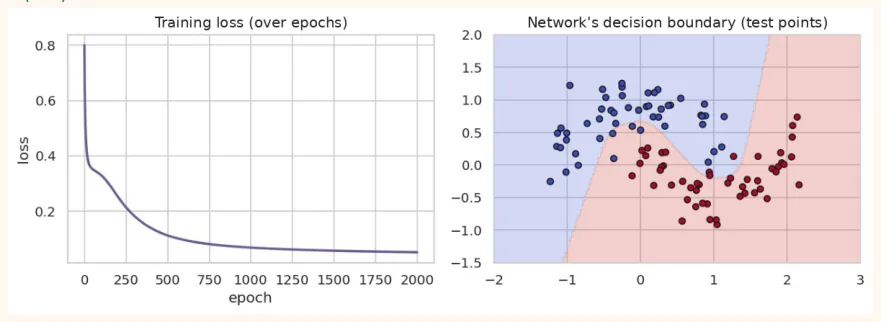
Now we put all the pieces above together and build a 2-layer network that will solve the make_moons (two curved moons) problem, which a straight line cannot solve.
from sklearn.datasets import make_moons
from sklearn.model_selection import train_test_split
X, y = make_moons(n_samples=400, noise=0.2, random_state=42)
X_train, X_test, y_train, y_test = train_test_split( X, y, test_size=0.25, random_state=42, stratify=y)
y_tr = y_train.reshape(-1, 1)
print("Train:", X_train.shape, " Test:", X_test.shape)
OUTPUT
Train:
(300, 2)  Test:
(100, 2)
np.random.seed(1)
n_hidden, lr, epochs = 8, 0.5, 2000
W1 = np.random.randn(2, n_hidden) * 0.5
b1 = np.zeros((1, n_hidden))
W2 = np.random.randn(n_hidden, 1) * 0.5
b2 = np.zeros((1, 1))
sigmoid = lambda z:
1 / (1 + np.exp(-z))
losses = []
for epoch in range(epochs):
    # ---- Forward ---Z1 = X_train @ W1 + b1
    A1 = np.tanh(Z1)
    Z2 = A1 @ W2 + b2
    A2 = sigmoid(Z2)
    loss = -np.mean(y_tr * np.log(A2 + 1e-9) + (1 - y_tr) * np.log(1 - A2 + 1e-9))
    losses.append(loss) # ---- Backward ---m = len(X_train)
    dZ2 = (A2 - y_tr) / m                 # the clean gradient of sigmoid + cross-entropy
    dW2 = A1.T @ dZ2
    db2 = dZ2.sum(axis=0, keepdims=True)
    dZ1 = (dZ2 @ W2.T) * (1 - A1 ** 2)    # derivative of tanh
    dW1 = X_train.T @ dZ1
    db1 = dZ1.sum(axis=0, keepdims=True) # ---- Update ---W1 -= lr * dW1
    b1 -= lr * db1 W2 -= lr * dW2
    b2 -= lr * db2
    if epoch % 400 == 0:
        print("epoch", epoch, " loss:", round(loss, 4))
        def predict(X):
        return (sigmoid(np.tanh(X @ W1 + b1) @ W2 + b2) > 0.5).astype(int).ravel()
print("Train accuracy:", round((predict(X_train) == y_train).mean(), 3))
print("Test accuracy :", round((predict(X_test) == y_test).mean(), 3))
OUTPUT epoch 0 loss: 0.8005 epoch 400 loss: 0.139 epoch 800 loss: 0.0778 epoch 1200 loss: 0.0626 epoch 1600 loss: 0.0557 Train accuracy: 0.977 Test accuracy : 0.93 Let us look at the loss curve and the decision boundary the network has learned:
fig, axes = plt.subplots(1, 2, figsize=(10, 3.6))
axes[0].plot(losses, color="#6B5B95", lw=2)
axes[0].set_title("Training loss (over epochs)")
axes[0].set_xlabel("epoch")
axes[0].set_ylabel("loss")
xx, yy = np.meshgrid(np.linspace(-2, 3, 200), np.linspace(-1.5, 2, 200))
grid = np.c_[xx.ravel(), yy.ravel()] axes[1].contourf(xx, yy, predict(grid).reshape(xx.shape), alpha=0.25, cmap="coolwarm") axes[1].scatter(X_test[:, 0], X_test[:, 1], c=y_test, cmap="coolwarm", edgecolor="k", s=25) axes[1].set_title("Network's decision boundary (test points)")
plt.tight_layout()
plt.show()
OUTPUT (chart)
21.8 Introduction to TensorFlow and Keras
Writing backprop by hand is good for understanding, but in real work we use TensorFlow . TensorFlow is Google's deep learning library, and Keras is its easy interface ( tf.keras ). It computes gradients by itself ( automatic differentiation ), runs on a GPU, and handles large models.
The 5-step Keras method
-
Build the model: a list of layers inside keras.Sequential([...]) .
-
Compile: tell it the optimizer, the loss and the metrics.
-
Fit: training with model.fit(X, y, epochs=..., validation_split=...) .
-
Evaluate: model.evaluate(X_test, y_test) .
-
Predict: model.predict(X_new) .
from tensorflow import keras
from tensorflow.keras import layers
model = keras.Sequential([
keras.Input(shape=(2,)),
layers.Dense(8, activation="relu"),     # hidden layer: 8 neurons
layers.Dense(1, activation="sigmoid"),  # output: probability
])
model.compile(optimizer="adam",
loss="binary_crossentropy",
metrics=["accuracy"])
model.summary() OUTPUT (sample) Model: "sequential" ┏━━━━━━━━━━━━━━━━━━━━━━━━━━━━━━━━━━━┳━━━━━━━━━━━━━━━━━━━━━━━━━━┳━━━━━━━━━━━━━━━━━┓ ┃ ┃ ┃ ┃ Layer (type) Output Shape Param # ┡━━━━━━━━━━━━━━━━━━━━━━━━━━━━━━━━━━━╇━━━━━━━━━━━━━━━━━━━━━━━━━━╇━━━━━━━━━━━━━━━━━┩ │ dense (Dense) │ (None, 8) │ 24 │ │ dense_1 (Dense) │ (None, 1) │ 9 │ └───────────────────────────────────┴──────────────────────────┴─────────────────┘
 Total params: 33 (132.00 B)
 Trainable params: 33 (132.00 B)
 Non-trainable params: 0 (0.00 B)
OUTPUT (sample)
Test accuracy: 0.950
First 5 probabilities: [0.88 0.26 0.22 0.14 0.06]
Actual labels        : [1 0 0 0 0]
Note: epoch means one complete pass over the whole training data, batch_size=32 means each update looks at 32 samples, and validation_split=0.2 keeps 20% of the training data aside for validation so that overfitting can be caught (Chapter 12).
You can also run a neural network with sklearn's MLPClassifier (this is also a real neural network), which lets you learn on your own laptop without Colab:
from sklearn.neural_network import MLPClassifier
mlp = MLPClassifier(hidden_layer_sizes=(8,), activation="relu", max_iter=2000, random_state=1)
mlp.fit(X_train, y_train)
print("sklearn MLP test accuracy:", round(mlp.score(X_test, y_test), 3))
print("Shapes of the layer weights:", [w.shape for w in mlp.coefs_])
OUTPUT sklearn MLP test accuracy: 0.95 Shapes of the layer weights: [(2, 8), (8, 1)]
21.9 Common Mistakes and Hands-on
Hands-on
-
Change the neurons: set n_hidden in the NumPy network to 2, 4, 16 and see how the decision boundary differs.
-
Change the activation: use ReLU instead of tanh in the hidden layer (derivative: 1 where z>0, otherwise 0).
-
Learning rate: set lr to 0.01, 0.5, 5 and compare the loss curves.
-
Change the dataset: run the same network on make_circles .
-
In Keras: change Dense(8) to Dense(32) and verify the Param # calculation in model.summary() yourself.
KEY TAKEAWAYS
-
Neuron = weighted sum + bias + activation. Only the weights and the bias are learned.
-
ReLU in hidden layers; sigmoid for binary; softmax for multiclass; linear output for regression.
-
Loss measures the network's error: MSE for regression, cross-entropy for classification.
-
Backpropagation = the gradient of every weight through the chain rule; then the update through gradient descent.
-
The 5 Keras steps: Sequential, compile, fit, evaluate, predict. Check the parameters with model.summary() .
-
A neural network is often no better than Random Forest on small table data; its strength lies in images, text and sequences.