Chapter 28: GANs and the Deep Learning Capstone Mini Project
MODULE 5 | WEEK 28
Chapter 28: GANs and the Deep Learning Capstone Mini Project
All the models so far recognized or estimated (classification, regression). Generative models go one step further: they create completely new data that looks like the real thing (new images, audio, text). In this chapter we will learn the GAN (Generative Adversarial Network) : a contest between two networks that makes each other better. Then we will do the Capstone Mini Project of Module 5, in which everything you have learned (ANN, CNN, regularization, evaluation) is joined into one complete project .
28.1 What are Generative models?
| Type | The question it solves | Example |
|---|---|---|
| Discriminative | Which class does this input belong to? (links y to x) | Is this picture a cat or a dog? |
| Generative | How do I makenewdata that looks like this class? | New faces, new images, new tunes |
An autoencoder (VAE) can become a generative model (Chapter 27). The GAN is a different and very famous way of reaching the same goal, which began with the paper by Ian Goodfellow in 2014.
28.2 The idea of a GAN: the counterfeiter and the police
Loss and the training steps
In every iteration two jobs are done in turn :
-
Train D: the target is 1 for real data and 0 for the fakes made by G (Binary Cross-Entropy).
-
Train G: show the fake data to D and set the target to 1 (G wants D to think it is real). At this time D's weights do not change , only G's.
D's loss:  -[ log D(real)  +  log(1 - D(G(z))) ]       <- D wants to reduce this
G's loss:  -log D(G(z))                                  <- G wants to reduce this
(non-saturating)
28.3 A real small GAN in NumPy (1D)
To understand the heart of a GAN we build the simplest GAN, whose data is just one number . Real data: a Normal distribution (mean = 4, std = 1.25). Generator: x = a*z + b (two parameters), where z is standard normal noise. Discriminator: a small logistic model that looks at x and x^2 . G has to learn that a = 1.25 and b = 4 are what is needed, but it is never told this ; it learns only from D's hints.
import numpy as np
import matplotlib.pyplot as plt
def sigmoid(s):
    return 1 / (1 + np.exp(-s))
def feats(x):
    return np.stack([x, x ** 2], axis=1)      # features for D
rng = np.random.RandomState(0)
REAL_MEAN, REAL_STD = 4.0, 1.25
a, b = 1.0, 0.0                    # Generator:
x = a*z + b   (bad at the start)
w, c = np.zeros(2), 0.0            # Discriminator:
D(x) = sigmoid(w . [x, x^2] + c)
lr_d, lr_g, batch = 0.05, 0.02, 64
history = []
for step in range(6000):
    # ---------- 1) Train the Discriminator ----------
    real = rng.normal(REAL_MEAN, REAL_STD, batch)
    fake = a * rng.randn(batch) + b
    D_real, D_fake = sigmoid(feats(real) @ w + c), sigmoid(feats(fake) @ w + c)
    grad_w = ((D_real - 1)[:, None] * feats(real)).mean(axis=0) + (D_fake[:, None] *
    feats(fake)).mean(axis=0)
    grad_c = (D_real - 1).mean() + D_fake.mean()
    w -= lr_d * grad_w
    c -= lr_d * grad_c
    # ---------- 2) Train the Generator (D's weights frozen) ----------
    z = rng.randn(batch)
    fake = a * z + b
    D_fake = sigmoid(feats(fake) @ w + c)
    dL_dx = -(1 - D_fake) * (w[0] + 2 * w[1] * fake)       # gradient of -log D(G(z))
    a -= lr_g * (dL_dx * z).mean()
    b -= lr_g * dL_dx.mean()
    history.append((a, b))
    history = np.array(history)
    last = history[-1000:]
    print("Real data      : mean =", REAL_MEAN, " std =", REAL_STD)
    print("Average of G's (a, b) over the last 1000 steps:", last.mean(axis=0).round(2))
    gen = history[-1, 0] * rng.randn(10000) + history[-1, 1]
    print("10000 samples from the Generator: mean =", gen.mean().round(2), " std =",
    gen.std().round(2))
OUTPUT
Real data      : mean = 4.0  std = 1.25
Average of G's (a, b) over the last 1000 steps: [1.28 3.38]
10000 samples from the Generator: mean = 3.86  std = 1.03
G learned to make the data without ever seeing the real parameters , only from D's hints: the mean of the generated data came out about 3.9 (real 4) and the std about 1.0 (real 1.25). Not perfect, but close to the real one. Let us see how a and b travelled during training, and finally the shape of the generated and the real data:
fig, axes = plt.subplots(1, 2, figsize=(10, 3.6))
axes[0].plot(history[:, 1], color="#6B5B95", lw=1, label="b (mean)")
axes[0].plot(history[:, 0], color="#A4457A", lw=1, label="a (std)")
axes[0].axhline(REAL_MEAN, color="#6B5B95", ls=":")
axes[0].axhline(REAL_STD,
color="#A4457A", ls=":")
axes[0].set_xlabel("training step")
axes[0].set_title("G's parameters (dotted = true
value)")
axes[0].legend()
real = rng.normal(REAL_MEAN, REAL_STD, 10000)
axes[1].hist(real, bins=50, density=True, alpha=0.6, color="gray", label="Real data")
axes[1].hist(gen, bins=50, density=True, alpha=0.6, color="#A4457A", label="Generator's
data")
axes[1].set_title("After training")
axes[1].legend()
plt.tight_layout()
plt.show()
OUTPUT (chart)
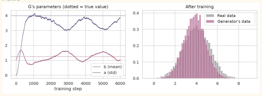
One important thing is visible: G's parameters do not go straight to the true value and stop , but keep oscillating around it . This is the real nature of GAN training: two networks are playing a minimax game , in which one's gain is the other's loss, which is why GAN training is hard and unstable .
28.4 Problems of GANs
| Problem | Meaning | Common remedy |
|---|---|---|
| Mode collapse | G makes only one or a few kinds of data (for example, only the digit 1) because that is what fools D | Minibatch features, WGAN loss, more diverse data |
| Unstable training | The losses jump around, sometimes D is too strong, sometimes G | A small learning rate for both (2e-4), Adam beta1 = 0.5, label smoothing |
| Problem | Meaning | Common remedy |
|---|---|---|
| Vanishing gradient for G | If D becomes too strong, G gets no learning signal | Non-saturating loss, do not let D learn far more than G |
| Hard to evaluate | There is no clear number like accuracy | Look at samples, FID score |
28.5 The structure of a GAN in Keras
We build a small GAN for Digits (8x8 = 64 pixels, 0 to 1). The Generator makes 64 pixels from 32 numbers of noise , and the Discriminator looks at 64 pixels and decides real/fake.
import tensorflow as tf
from tensorflow import keras
from tensorflow.keras import layers
latent_dim = 32
generator = keras.Sequential([
keras.Input(shape=(latent_dim,)),
layers.Dense(128), layers.LeakyReLU(0.2),
layers.Dense(64, activation="sigmoid"),          # 64 pixels, 0 to 1
], name="generator")
discriminator = keras.Sequential([
keras.Input(shape=(64,)),
layers.Dense(128), layers.LeakyReLU(0.2),
layers.Dropout(0.3),
layers.Dense(1, activation="sigmoid"),           # real (1) or fake (0)
], name="discriminator")
generator.summary() discriminator.summary() OUTPUT (sample) Model: "generator"
┏━━━━━━━━━━━━━━━━━━━━━━━━━━━━━━━━━━━┳━━━━━━━━━━━━━━━━━━━━━━━━━━┳━━━━━━━━━━━━━━━━━┓
┃
┃
┃
┃
 Layer (type)                       Output Shape                      Param #
┡━━━━━━━━━━━━━━━━━━━━━━━━━━━━━━━━━━━╇━━━━━━━━━━━━━━━━━━━━━━━━━━╇━━━━━━━━━━━━━━━━━┩
│ dense (Dense)                     │ (None, 128)              │           4,224 │
│ leaky_re_lu (LeakyReLU)           │ (None, 128)              │               0 │
│ dense_1 (Dense)                   │ (None, 64)               │           8,256 │
└───────────────────────────────────┴──────────────────────────┴─────────────────┘
 Total params: 12,480 (48.75 KB)
 Trainable params: 12,480 (48.75 KB)
 Non-trainable params: 0 (0.00 B)
Model: "discriminator"
┏━━━━━━━━━━━━━━━━━━━━━━━━━━━━━━━━━━━┳━━━━━━━━━━━━━━━━━━━━━━━━━━┳━━━━━━━━━━━━━━━━━┓
┃
┃
┃
┃
 Layer (type)                       Output Shape                      Param #
┡━━━━━━━━━━━━━━━━━━━━━━━━━━━━━━━━━━━╇━━━━━━━━━━━━━━━━━━━━━━━━━━╇━━━━━━━━━━━━━━━━━┩
│ dense_2 (Dense)                   │ (None, 128)              │           8,320 │
│ leaky_re_lu_1 (LeakyReLU)         │ (None, 128)              │               0 │
│ dropout (Dropout)                 │ (None, 128)              │               0 │
│ dense_3 (Dense)                   │ (None, 1)                │             129 │
└───────────────────────────────────┴──────────────────────────┴─────────────────┘
 Total params: 8,449 (33.00 KB)
 Trainable params: 8,449 (33.00 KB)
 Non-trainable params: 0 (0.00 B)
28.6 Other generative models
| Model | Idea | Pros | Cons |
|---|---|---|---|
| VAE | Encoder-decoder, the code is a distribution | Stable training, a clean latent space | The samples are often blurry |
| GAN | A contest between G and D | Fast, sharp and clear samples | Hard training, mode collapse |
| Diffusion | Start from noise and clean it up step by step | The best quality and variety (today's image-making AI) | Generating a sample is slow |
| LLM (Transformer) | Predict the next word (Module 6) | Text, code, and much more | Huge compute |
Today's image-making tools are mostly built on diffusion models , and for text on Transformers/LLMs (our next module). But the GAN idea has always remained important: a contest between two networks and adversarial training, which is still useful in security, robustness and creating data .
28.7 Capstone Mini Project: a handwritten digit recognition system
This is the mini project of Module 5, which shows the full skeleton of a complete data science project. The goal: recognize a digit from an image and do the whole job in a professional way: problem, data, baseline, model, tuning, evaluation, error analysis, save, and report.
| Stage | What to do | Chapter |
|---|---|---|
| 1. Problem statement | Decide the goal and the success metric (for example accuracy >= 97%) | Module 1 |
| 2. Understanding the data (EDA) | Shape, count of classes, look at the images | Chapter 23 |
| 3. Preparation | Train/validation/test, scaling | Chapter 22 |
| 4. Baselines | Simple models (Logistic, Random Forest, SVM) | Module 4 |
| 5. Neural Network / CNN | ANN, then CNN, regularization, callbacks | Chapters 21 to 24 |
| 6. Evaluation | Test accuracy, confusion matrix, error analysis | Chapter 24 |
| 7. Save and predict function | Save the model, predict on new data | Chapter 24 |
| 8. Report | Results, mistakes, future work | Below |
Stages 1 to 3: Problem, data and preparation
Problem statement:
"Build a model that recognizes a digit (0 to 9) from an 8x8 greyscale image. Success metric: test accuracy >= 97%, and recall of every class >= 90%."
import numpy as np
import matplotlib.pyplot as plt
from sklearn.datasets import load_digits
from sklearn.model_selection import train_test_split
digits = load_digits()
X, y = digits.data / 16.0, digits.target
print("Images:", X.shape[0], "| Pixels:", X.shape[1], "| Classes:", len(np.unique(y)))
print("Count of each class:", np.bincount(y)) # Train 60% / Validation 20% / Test 20%
X_tr, X_tmp, y_tr, y_tmp = train_test_split(X, y, test_size=0.4, random_state=42, stratify=y)
X_val, X_te, y_val, y_te = train_test_split(X_tmp, y_tmp, test_size=0.5, random_state=42, stratify=y_tmp)
print("Train:", X_tr.shape, " Validation:", X_val.shape, " Test:", X_te.shape)
fig, axes = plt.subplots(2, 10, figsize=(10, 2.4))
for d in range(10):
    for r in range(2):
        axes[r, d].imshow(digits.images[np.where(y == d)[0][r]], cmap="gray_r", interpolation="nearest") axes[r, d].axis("off") axes[0, d].set_title(str(d), fontsize=9)
        plt.tight_layout()
        plt.show()
OUTPUT
Images:
1797 | Pixels:
64 | Classes:
10 Count of each class:
[178 182 177 183 181 182 181 179 174 180] Train:
(1078, 64)  Validation:
(359, 64)  Test:
(360, 64)
OUTPUT (chart)
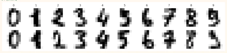
We have set aside the test set right now . We will use it only once, at the very end . For choosing a model there is the validation set.
Stages 4 and 5: From a baseline to a neural network
import warnings
warnings.filterwarnings("ignore")
from sklearn.linear_model import LogisticRegression
from sklearn.ensemble import RandomForestClassifier
from sklearn.svm import SVC
from sklearn.neural_network import MLPClassifier
candidates = {
"Logistic Regression": LogisticRegression(max_iter=3000),
"Random Forest": RandomForestClassifier(n_estimators=200, random_state=0),
"SVM (RBF)": SVC(),
"Neural Net (64,)": MLPClassifier(hidden_layer_sizes=(64,), max_iter=500,
random_state=0),
"Neural Net (128,64) + early stop":
MLPClassifier(hidden_layer_sizes=(128, 64), early_stopping=True, n_iter_no_change=10, max_iter=500, random_state=0), }
print("Model".ljust(34), "Train acc   Validation acc")
results = {}
for name, m in candidates.items():
    m.fit(X_tr, y_tr) results[name] = m
    print(name.ljust(34), str(round(m.score(X_tr, y_tr), 3)).ljust(11), round(m.score(X_val, y_val), 3))
OUTPUT Model Train acc Validation acc Logistic Regression 0.985 0.958 Random Forest 1.0 0.972 SVM (RBF) 0.998 0.986 Neural Net (64,) 1.0 0.972 Neural Net (128,64) + early stop 0.987 0.961 Choose the model by looking at the validation accuracy in this table (not the test!). A large gap between train and validation accuracy is a sign of overfitting (Chapter 22).
best_name = max(results, key=lambda n: results[n].score(X_val, y_val))
best = results[best_name]
print("Best model on validation:", best_name)
from sklearn.metrics import classification_report, confusion_matrix
import seaborn as sns
pred = best.predict(X_te)                       # the FIRST and LAST use of the test set
print("Test accuracy:", round((pred == y_te).mean(), 3))
print()
print(classification_report(y_te, pred, digits=3))
cm = confusion_matrix(y_te, pred)
fig, ax = plt.subplots(figsize=(5.6, 4.6))
sns.heatmap(cm, annot=True, fmt="d", cmap="Purples", cbar=False, ax=ax)
ax.set_xlabel("Predicted")
ax.set_ylabel("Actual")
ax.set_title("Test set: confusion matrix")
plt.show()
OUTPUT Best model on validation: SVM (RBF) Test accuracy: 0.986
              precision    recall  f1-score   support
           0      1.000     0.971     0.986        35
           1      0.974     1.000     0.987        37
           2      1.000     1.000     1.000        35
           3      1.000     1.000     1.000        37
           4      0.973     1.000     0.986        36
           5      1.000     1.000     1.000        37
           6      1.000     1.000     1.000        36
           7      0.923     1.000     0.960        36
           8      1.000     0.971     0.986        35
           9      1.000     0.917     0.957        36
    accuracy                          0.986       360
   macro avg      0.987     0.986     0.986       360
weighted avg      0.987     0.986     0.986       360
OUTPUT (chart)
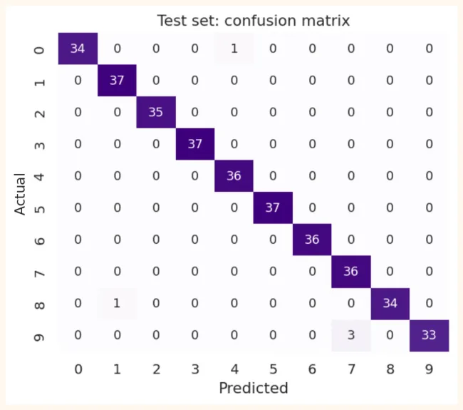
This result is checked against our success metric (accuracy 97% and recall of every class 90%). In this run the test accuracy is 98.6% and the lowest recall (digit 9) is 91.7% , so both conditions are met. If they are not met, do error analysis (Chapter 24: look at the wrong images) and improve the model/data.
Stage 5 (continued): the final CNN code in Keras (Colab)
The CNN below is the same one you learned in Chapter 23, just in the shape of a complete project with Dropout, callbacks and augmentation :
import numpy as np
from tensorflow import keras
from tensorflow.keras import layers, callbacks
X_tr_img = X_tr.reshape(-1, 8, 8, 1)
X_val_img = X_val.reshape(-1, 8, 8, 1)
X_te_img = X_te.reshape(-1, 8, 8, 1)
cnn = keras.Sequential([
keras.Input(shape=(8, 8, 1)),
layers.RandomTranslation(0.1, 0.1),                  # augmentation (during training
only)
layers.Conv2D(16, 3, padding="same", activation="relu"),
layers.BatchNormalization(),
layers.MaxPooling2D(),
layers.Conv2D(32, 3, padding="same", activation="relu"),
layers.MaxPooling2D(),
layers.Flatten(),
layers.Dropout(0.3),
layers.Dense(64, activation="relu"),
layers.Dense(10, activation="softmax"),
])
cnn.compile(optimizer=keras.optimizers.Adam(1e-3),
loss="sparse_categorical_crossentropy", metrics=["accuracy"])
cb = [callbacks.EarlyStopping(patience=12, restore_best_weights=True),
callbacks.ReduceLROnPlateau(factor=0.5, patience=5),
callbacks.ModelCheckpoint("best_digits_cnn.keras", save_best_only=True)]
history = cnn.fit(X_tr_img, y_tr, validation_data=(X_val_img, y_val),
epochs=200, batch_size=32, callbacks=cb, verbose=0)
test_loss, test_acc = cnn.evaluate(X_te_img, y_te, verbose=0)    # test only now, once
print("CNN test accuracy:", round(test_acc, 3))
Run this cell in Colab, write down your test accuracy and compare it with the sklearn model above. Write both results in your report (the better one is the final model, but both must be mentioned).
Stage 7: Save and a predict function
model = keras.models.load_model("best_digits_cnn.keras")
def predict_digit(image_8x8):
    """image_8x8: an 8x8 numpy array, pixels 0 to 16"""
    x = (np.asarray(image_8x8, dtype="float32") / 16.0).reshape(1, 8, 8, 1)   # the same preprocessing as in training
    probs = model.predict(x, verbose=0)[0]
    return {"digit": int(probs.argmax()), "confidence": round(float(probs.max()), 3)}
print(predict_digit(digits.images[0]))
28.8 Project Report and Marking Rubric
The project report should have these parts:
-
Title and goal: what the problem is and why it matters.
-
Introduction to the data: count, shape, classes, some images.
-
Method: preprocessing, the split (60/20/20), the models you tried.
-
Results: a table of validation and test accuracy, the confusion matrix, charts.
-
Error analysis: where the model makes mistakes and why.
-
Conclusion and future work: what was learned, what could be better (more data, augmentation, Transfer Learning).
-
Ethics and limits: where the model will not work (for example different handwriting, bigger images).
| Part | Marks |
|---|---|
| Understanding of the problem and data | 10 |
| Preprocessing and a correct split (no leakage) | 15 |
| Baselines and model comparison | 20 |
| Performance of the neural network / CNN | 20 |
| Evaluation and error analysis | 20 |
| Clean code and clarity of the report | 15 |
| Total | 100 |
28.9 Module 5 Summary
| Chapter | What you learned |
|---|---|
| 21 | Neuron, activation, loss, backpropagation, the 5 steps of Keras |
| Chapter | What you learned |
|---|---|
| 22 | Cures for overfitting (Dropout, L2, Early Stopping, BatchNorm), initialization, optimizers |
| 23 | CNN: convolution, pooling, counting parameters |
| 24 | The ideas of ResNet and MobileNet, Transfer Learning, an image project |
| 25 | RNN, LSTM, GRU, turning text into numbers |
| 26 | Time series: baselines, windowing, differencing, walk-forward validation |
| 27 | Autoencoders, comparison with PCA, denoising, anomaly detection |
| 28 | GAN, generative models, the capstone mini project |
In Module 6 you will learn Transformers and Attention , on which LLMs like ChatGPT are built, and then you will build AI applications yourself with the OpenAI API .
28.10 Common Mistakes and Hands-on
Hands-on
-
NumPy GAN: change the real data's mean from 4 to 8 and std from 1.25 to 2; look at G's (a, b) again.
-
Learning rate: set lr_g to 0.002 and 0.2 and write down the difference in training.
-
Generated samples: train the Keras GAN in Colab and make a picture of 16 samples every 50 epochs.
-
Capstone: add one more model (for example KNN or Gradient Boosting) to the project above and update the validation table.
-
Report: write a 2-page report of this project according to the rubric.
KEY TAKEAWAYS
-
Generative models create new data; discriminative models recognize or estimate.
-
GAN: the Generator (makes fakes) and the Discriminator (tells real from fake) get better by competing with each other.
-
G is trained with the non-saturating loss (-log D(G(z))); in training both are updated in turn.
-
GAN training is unstable (oscillation, mode collapse); judge it by looking at samples, not by the loss.
-
Adam(2e-4, beta1=0.5), LeakyReLU and label smoothing are common GAN recipes.
-
Diffusion models and LLMs are today's big generative models; VAEs and GANs paved the way.
-
The skeleton of a capstone: problem, EDA, split, baselines, model, evaluation, error analysis, save, report.
-
Use the test set only once at the end; choose the model from the validation set.
-
For things like deepfakes, keep ethics and permission in mind.