Chapter 26: Time Series Forecasting
MODULE 5 | WEEK 26
Chapter 26: Time Series Forecasting
Time series is data that is recorded over time : daily sales, monthly electricity consumption, hourly weather, the price of a share. In business the most frequently asked question is: "What will happen in the future?" In this chapter we will learn the real principles of forecasting : never breaking the time order, building a baseline , turning a time series into supervised learning through windowing , and then forecasting with ML and LSTM/GRU .
26.1 What is a Time Series?
In a time series, every observation has a time attached, and nearby observations are linked to each other (today's sales resemble yesterday's sales). This is why the usual ML rules (random shuffling) do not work here.
We will build a synthetic series that still looks like real life: 10 years (120 months) of sales of a shop, with a rising trend , a yearly seasonal effect (seasonality) and a little noise . The benefit of synthetic data is that we know what is hidden inside.
import numpy as np
import pandas as pd
import matplotlib.pyplot as plt
rng = np.random.RandomState(42)
months = pd.date_range("2015-01-01", periods=120, freq="MS")    # the first day of every month tareekh
t = np.arange(120)
trend = 100 + 0.8 * t                          # rising a little every month
season = 15 * np.sin(2 * np.pi * t / 12)       # one cycle in 12 months
noise = rng.normal(0, 3, 120)
sales = trend + season + noise
ts = pd.Series(sales, index=months, name="sales")
print(ts.head(4).round(1))
print("Total months:", len(ts), "| Min:", ts.min().round(1), "| Max:", ts.max().round(1))
fig, ax = plt.subplots(figsize=(10, 3.6))
ax.plot(ts, color="#6B5B95", lw=1.8)
ax.set_title("Monthly sales (synthetic data): trend + seasonality + noise")
ax.set_ylabel("sales")
plt.show()
OUTPUT 2015-01-01 101.5 2015-02-01 107.9 2015-03-01 116.5
2015-04-01 122.0 Freq: MS, Name: sales, dtype: float64 Total months: 120 | Min: 92.0 | Max: 205.3 OUTPUT (chart)
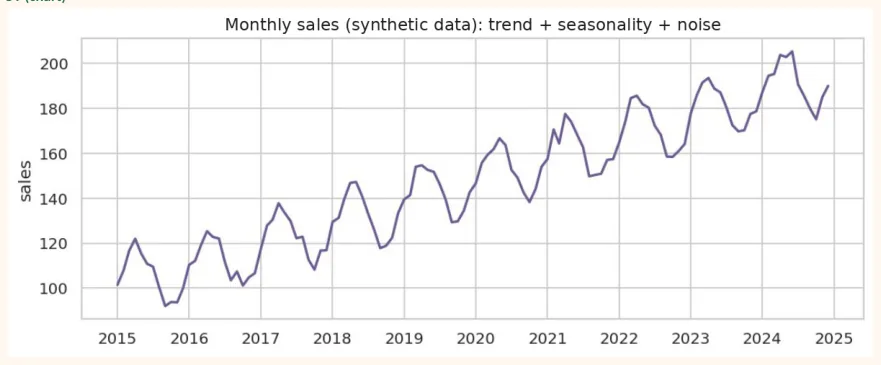
| Part | Meaning | In this series |
|---|---|---|
| Trend | A long-term upward or downward movement | An increase of +0.8 every month |
| Seasonality | A repeating seasonal pattern | The same shape after every 12 months |
| Noise | Irregular small ups and downs | Random noise (std = 3) |
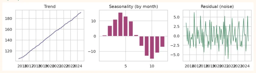
Separating these parts from the real series ( decomposition ) is the very first step:
trend_est = ts.rolling(window=12, center=True).mean()          # 12-month
average =
trend
detrended = ts - trend_est
season_est = detrended.groupby(detrended.index.month).mean()     # the usual effect of each month
print("Seasonal effect of each month (first 6 months):")
print(season_est.round(1).head(6))
print("Month with the largest effect:", int(season_est.idxmax()), " | smallest:",
int(season_est.idxmin()))
fig, axes = plt.subplots(1, 3, figsize=(10, 2.8)) axes[0].plot(ts.index, trend_est, color="#6B5B95")
axes[0].set_title("Trend") axes[1].bar(season_est.index, season_est.values, color="#A4457A")
axes[1].set_title("Seasonality (by month)") axes[2].plot(ts.index, (detrended - detrended.index.month.map(season_est)), color="#2F7D4F", lw=1) axes[2].set_title("Residual (noise)")
plt.tight_layout()
plt.show()
OUTPUT Seasonal effect of each month (first 6 months): 1 0.6 2 6.8 3 10.9 4 15.6 5 13.0 6 9.8 Name: sales, dtype: float64 Month with the largest effect: 4 | smallest: 10
OUTPUT (chart)
26.2 The golden rules of forecasting
26.3 Baseline models and Metrics
| Baseline | Idea |
|---|---|
| Naive | Next month's sales = last month's sales |
| Seasonal Naive | Next month's sales = the sales ofthe same month last year |
| Moving Average | The average of the last 12 months |
| Metric | Formula (short) Meaning |
|---|---|
| MAE | mean(|actual - forecast|) Average error, in the same unit as the data |
| RMSE | sqrt(mean((actual - forecast)^2)) Punishes large errors more |
| MAPE | mean(|actual - forecast| / |actual|) x 100 Error in percent (wrong if the actual is near 0) |
def metrics(y_true, y_pred):
    y_true, y_pred = np.asarray(y_true), np.asarray(y_pred)
    mae = np.mean(np.abs(y_true - y_pred))
    rmse = np.sqrt(np.mean((y_true - y_pred) ** 2))
    mape = np.mean(np.abs((y_true - y_pred) / y_true)) * 100
    return round(mae, 2), round(rmse, 2), round(mape, 2)

full = ts.values
n_tr = len(train)
y_test = test.values
# One-step baselines: the previous ACTUAL values are used for every test month
naive = full[n_tr - 1:-1]                                  # the previous month
seasonal_naive = full[n_tr - 12:-12]                       # 12 months earlier
moving_avg = np.array([full[i - 12:i].mean() for i in range(n_tr, len(full))])
print("Baseline".ljust(16), "MAE    RMSE   MAPE%")
for name, pred in [("Naive", naive), ("Seasonal naive", seasonal_naive),
                   ("Moving avg (12)", moving_avg)]:
    print(name.ljust(16), *metrics(y_test, pred))
OUTPUT
Baseline         MAE    RMSE   MAPE%
Naive            5.65 6.78 3.05
Seasonal naive   10.03 10.67 5.39
Moving avg (12)  9.8 11.77 5.16
These numbers are our line to beat . Any model that cannot beat them is not needed.
26.4 Windowing: turning a time series into supervised learning
An ML model needs (X, y) . In a time series we take the previous window steps as X and the next step as y . This method is called a sliding window .
Example window
Series: 10, 12, 11, 14, 15, 17, 16
Window: 3
[10, 12, 11] -> 14
[12, 11, 14] -> 15
[11, 14, 15] -> 17
[14, 15, 17] -> 16
def make_windows(values, window):
    X, y = [], []
    for i in range(window, len(values)):
        X.append(values[i - window:i])
        y.append(values[i])
    return np.array(X), np.array(y)

demo = np.array([10, 12, 11, 14, 15, 17, 16], dtype=float)
Xd, yd = make_windows(demo, 3)
print(Xd)
print("y:", yd)
print("X shape:", Xd.shape, " y shape:", yd.shape)
OUTPUT
[[10. 12. 11.]
 [12. 11. 14.]
 [11. 14. 15.]
 [14. 15. 17.]]
y: [14. 15. 17. 16.]
X shape: (4, 3)  y shape: (4,)
RNN/LSTM/GRU need 3D input: (samples, timesteps, features) . Our series has only 1 feature (sales):
Xd3 = Xd.reshape(Xd.shape[0], Xd.shape[1], 1)
print("Shape for an RNN:", Xd3.shape, "-> (samples, timesteps, features)")
OUTPUT Shape for an RNN: (4, 3, 1) -> (samples, timesteps, features)
26.5 Scaling and the full preparation
Neural networks need scaled data. The scaler is fitted on the train data only (otherwise future information would leak):
from sklearn.preprocessing import MinMaxScaler
window = 12
scaler = MinMaxScaler().fit(train.values.reshape(-1, 1))            # on train only
scaled = scaler.transform(ts.values.reshape(-1, 1)).ravel()
X_all, y_all = make_windows(scaled, window) # the target of a window is the month at index (window + i)
target_idx = np.arange(window, len(scaled))
is_test = target_idx >= n_tr                       # those whose target is in the test period
X_tr, y_tr = X_all[~is_test], y_all[~is_test]
X_te, y_te = X_all[is_test], y_all[is_test]
print("Train windows:", X_tr.shape, " Test windows:", X_te.shape)
print("Scaled train range:", scaled[:n_tr].min().round(2), "to", scaled[:n_tr].max().round(2))
print("Scaled test range :", scaled[n_tr:].min().round(2), "to", scaled[n_tr:].max().round(2))
OUTPUT Train windows: (84, 12) Test windows: (24, 12) Scaled train range: 0.0 to 1.0 Scaled test range : 0.83 to 1.21 REMEMBER
The scaled range of the test went above 1 , because the series is rising and the train data simply did not have such large values. This is perfectly fine (there is no leakage), but it means that the model will have to extrapolate outside the train range . This is the real problem with series that have a trend.
26.6 Forecasting with ML and a Neural Network
Three models: Ridge Regression (linear), Random Forest , and a small neural network ( MLPRegressor , a real neural net). All three are given the same previous 12 months:
from sklearn.linear_model import Ridge
from sklearn.ensemble import RandomForestRegressor
from sklearn.neural_network import MLPRegressor
import warnings
warnings.filterwarnings("ignore")
models = {
"Ridge": Ridge(alpha=0.1),
"Random Forest": RandomForestRegressor(n_estimators=200, random_state=0),
"Neural Net (MLP)": MLPRegressor(hidden_layer_sizes=(32, 16), max_iter=3000,
random_state=0),
}
preds = {}
print("Model".ljust(18), "MAE    RMSE   MAPE%")
for name, m in models.items():
    m.fit(X_tr, y_tr)
    p_scaled = m.predict(X_te)
    p = scaler.inverse_transform(p_scaled.reshape(-1, 1)).ravel()   # back to the original unit
    preds[name] = p
    print(name.ljust(18), *metrics(y_test, p))
OUTPUT
Model              MAE    RMSE   MAPE%
Ridge              2.62 3.42 1.4
Random Forest      7.76 9.95 4.04
Neural Net (MLP)   8.59 10.08 4.67
fig, ax = plt.subplots(figsize=(10, 3.8))
ax.plot(train.index[-36:], train.values[-36:], color="gray", lw=1.5, label="Train (last 3 years)")
ax.plot(test.index, y_test, color="black", lw=2, label="Actual (test)")
cols = {"Ridge": "#6B5B95", "Random Forest": "#B7791F", "Neural Net (MLP)": "#A4457A"}
for name, p in preds.items():
    ax.plot(test.index, p, color=cols[name], lw=1.6, ls="--", label=name)
ax.set_title("One-step forecast: test period")
ax.legend(ncol=2, fontsize=8)
plt.show()
OUTPUT (chart)
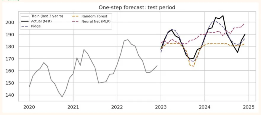
Notice that Ridge (linear) came out the best, and Random Forest and Neural Net both stayed behind even the naive baseline. The reason: a Random Forest gives the average of values it saw in training inside its trees, so it cannot extrapolate beyond the largest value of the train data ; a neural net is also weak outside the train range. A linear model catches the trend directly.
Differencing: remove the trend and try again
diff = np.diff(ts.values)                              # the change of every month
d_tr_end = n_tr - 1                                    # this many elements of diff are train
sc2 = MinMaxScaler().fit(diff[:d_tr_end].reshape(-1, 1))
d_scaled = sc2.transform(diff.reshape(-1, 1)).ravel()
Xd_all, yd_all = make_windows(d_scaled, window)
d_target_idx = np.arange(window, len(d_scaled))        # indices of diff
is_test_d = d_target_idx >= d_tr_end
Xd_tr, yd_tr = Xd_all[~is_test_d], yd_all[~is_test_d]
Xd_te, yd_te = Xd_all[is_test_d], yd_all[is_test_d]
print("Differenced train windows:", Xd_tr.shape, " test windows:", Xd_te.shape)
prev_values = full[n_tr - 1:-1]                         # the previous ACTUAL value (to add the
change back to)
for name, m in [("Random Forest (diff)", RandomForestRegressor(n_estimators=200, random_state=0)), ("Neural Net (diff)", MLPRegressor(hidden_layer_sizes=(32, 16), max_iter=3000, random_state=0)), ("Ridge (diff)", Ridge(alpha=0.1))]:
    m.fit(Xd_tr, yd_tr)
    d_pred = sc2.inverse_transform(m.predict(Xd_te).reshape(-1, 1)).ravel()
    p = prev_values + d_pred                            # previous value + predicted change preds[name] = p
    print(name.ljust(22), *metrics(y_test, p))
OUTPUT Differenced train windows: (83, 12) test windows: (24, 12) Random Forest (diff) 3.42 4.14 1.83 Neural Net (diff) 3.36 4.71 1.8 Ridge (diff) 2.89 3.54 1.54 After differencing, the RMSE of both Random Forest and Neural Net came down from around 10 to around 4 , because now the model does not have to learn the trend, only the change and the seasonality , which have already been seen in the train range. (In this series Ridge still remains simple and strong.)
26.7 Multi-step forecast: several months ahead
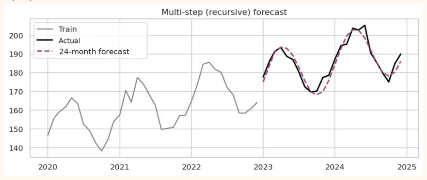
So far we predicted one step ahead (one-step) and gave the actual previous values every time. In real life we often need several months ahead , when the actual values are not known. The recursive method: make the first forecast, add it to the window, and make the next one.
rm = Ridge(alpha=0.1).fit(X_tr, y_tr)               # a model learned on the train windows
history = list(scaled[:n_tr])                         # only the data up to the train end is known
forecast = []
for step in range(test_size):
    x = np.array(history[-window:]).reshape(1, -1)
    p = rm.predict(x)[0]
    forecast.append(p)
    history.append(p)                                 # its own prediction becomes the next step
    input
    forecast = scaler.inverse_transform(np.array(forecast).reshape(-1, 1)).ravel()
    print("24-month recursive forecast (Ridge):", *metrics(y_test, forecast))
    print("Naive (repeat last value, baseline):", *metrics(y_test, [full[n_tr - 1]] * test_size))
    fig, ax = plt.subplots(figsize=(10, 3.6))
    ax.plot(train.index[-36:], train.values[-36:], color="gray", lw=1.5, label="Train")
    ax.plot(test.index, y_test, color="black", lw=2, label="Actual")
    ax.plot(test.index, forecast, color="#A4457A", lw=2, ls="--", label="24-month forecast")
    ax.set_title("Multi-step (recursive) forecast")
    ax.legend()
    plt.show()
OUTPUT 24-month recursive forecast (Ridge): 2.48 3.17 1.33 Naive (repeat last value, baseline): 22.04 24.15 11.59
OUTPUT (chart)
26.8 Walk-forward Validation (TimeSeriesSplit)
In time series K-Fold (with shuffling) is wrong. The right method: old data for training, the data after it for validation , and each time make the train part a little longer.
from sklearn.model_selection import TimeSeriesSplit
tscv = TimeSeriesSplit(n_splits=4, test_size=12)
for k, (tr_idx, va_idx) in enumerate(tscv.split(X_tr), 1):
    m = Ridge(alpha=0.1).fit(X_tr[tr_idx], y_tr[tr_idx])
    p = m.predict(X_tr[va_idx])
    rmse = np.sqrt(np.mean((y_tr[va_idx] - p) ** 2))
    print("Fold", k, "| train:", tr_idx[0], "to", tr_idx[-1], "| validate:", va_idx[0], "to", va_idx[-1], "| RMSE (scaled):", round(rmse, 4))
OUTPUT Fold 1 | train: 0 to 35 | validate: 36 to 47 | RMSE (scaled): 0.0302 Fold 2 | train: 0 to 47 | validate: 48 to 59 | RMSE (scaled): 0.0298 Fold 3 | train: 0 to 59 | validate: 60 to 71 | RMSE (scaled): 0.0437 Fold 4 | train: 0 to 71 | validate: 72 to 83 | RMSE (scaled): 0.0305
26.9 LSTM, GRU and Conv1D forecasting in Keras
Now the same problem in Keras. The input shape is (window, 1) . The data is just the X_tr of the previous section; we only need to add an axis for one feature.
import numpy as np
from tensorflow import keras
from tensorflow.keras import layers
X_tr3 = X_tr.reshape(-1, 12, 1)          # (samples, 12 timesteps, 1 feature)
X_te3 = X_te.reshape(-1, 12, 1)
lstm_model = keras.Sequential([ keras.Input(shape=(12, 1)), layers.LSTM(32), layers.Dense(1),                     # regression: no activation ])
lstm_model.compile(optimizer="adam", loss="mse")
lstm_model.summary()
OUTPUT (sample) Model: "sequential" ┏━━━━━━━━━━━━━━━━━━━━━━━━━━━━━━━━━━━┳━━━━━━━━━━━━━━━━━━━━━━━━━━┳━━━━━━━━━━━━━━━━━┓ ┃ ┃ ┃ ┃ Layer (type) Output Shape Param # ┡━━━━━━━━━━━━━━━━━━━━━━━━━━━━━━━━━━━╇━━━━━━━━━━━━━━━━━━━━━━━━━━╇━━━━━━━━━━━━━━━━━┩ │ lstm (LSTM) │ (None, 32) │ 4,352 │ │ dense (Dense) │ (None, 1) │ 33 │ └───────────────────────────────────┴──────────────────────────┴─────────────────┘
 Total params: 4,385 (17.13 KB)
 Trainable params: 4,385 (17.13 KB)
 Non-trainable params: 0 (0.00 B)
OUTPUT (sample)
3393 161
26.10 Common Mistakes and Hands-on
Hands-on
-
Change the series: raise the noise std from 3 to 10 and see which model stays the best.
-
Change the window: try 6, 12, 24 and write down the comparison of RMSE.
-
Remove the seasonality: take the seasonal part out of the series and see how the baselines change.
-
Your own data: write down 24 months of your home's electricity bill (or any data of your own) and build a seasonal naive baseline.
-
Keras: in Colab, make a table of the parameters, time and RMSE of LSTM, GRU and Conv1D.
KEY TAKEAWAYS
-
Time series = trend + seasonality + noise. Never break the order; no shuffling.
-
Always a baseline first: naive, seasonal naive, moving average.
-
Metrics: MAE, RMSE, MAPE. Measure after bringing scaled values back to the original unit.
-
Use windowing to turn the series into (X, y); the shape for an RNN is (samples, timesteps, features).
-
Fit the scaler on train only. The test range can fall outside the train range.
-
On a series with a trend, differencing makes tree-based models work fine too.
-
Multi-step: recursive (errors add up) or direct.
-
Validation: TimeSeriesSplit / walk-forward, never shuffled K-Fold.