Chapter 22: Advanced Neural Networks and Optimization Techniques
MODULE 5 | WEEK 22
Chapter 22: Advanced Neural Networks and Optimization Techniques
In the last chapter you built a small network. In real problems networks are deep , and training them is an art : the loss gets stuck, the network overfits , or training becomes very slow. In this chapter we will learn how to make a network better : deep networks, protection from overfitting ( L2, Dropout, Early Stopping, Batch Normalization ), proper weight initialization , and optimizers ( SGD, Momentum, RMSprop, Adam ) that make training faster and more stable.
22.1 Deep networks and multiclass classification
In this chapter we will use a real dataset: Digits (seen in Chapter 8). It has 8x8 images of 1797 handwritten digits (0 to 9), so each image has 64 pixels (from 0 to 16). This is multiclass classification : 10 classes, so the last layer has 10 neurons and softmax .
import numpy as np
from sklearn.datasets import load_digits
from sklearn.model_selection import train_test_split
from sklearn.preprocessing import StandardScaler
digits = load_digits()
X, y = digits.data, digits.target
print("X shape:", X.shape, " classes:", np.unique(y))
X_tr, X_te, y_tr, y_te = train_test_split(X, y, test_size=0.25, random_state=42, stratify=y)
scaler = StandardScaler().fit(X_tr)          # fit on train only (no leakage)
X_tr_s, X_te_s = scaler.transform(X_tr), scaler.transform(X_te)
print("Train:", X_tr_s.shape, " Test:", X_te_s.shape)
OUTPUT X shape: (1797, 64) classes: [0 1 2 3 4 5 6 7 8 9] Train: (1347, 64) Test: (450, 64) Now let us try networks of different depths . sklearn's MLPClassifier is also a real neural network (backprop + gradient descent), so these results are real:
from sklearn.neural_network import MLPClassifier
for layers in [(), (16,), (64,), (128, 64), (128, 64, 32)]:
    if layers == ():
        from sklearn.linear_model import LogisticRegression
        m = LogisticRegression(max_iter=2000)
        name = "No hidden layer (Logistic)"
    else:
        m = MLPClassifier(hidden_layer_sizes=layers, max_iter=500, random_state=0)
        name = "Hidden layers " + str(layers)
        m.fit(X_tr_s, y_tr)
        print(name.ljust(34), "test accuracy:", round(m.score(X_te_s, y_te), 3))
OUTPUT
No hidden layer (Logistic)         test accuracy: 0.978
Hidden layers (16,)                test accuracy: 0.958
Hidden layers (64,)                test accuracy: 0.978
Hidden layers (128, 64)            test accuracy: 0.98
Hidden layers (128, 64, 32)        test accuracy: 0.976
22.2 Overfitting in a neural network
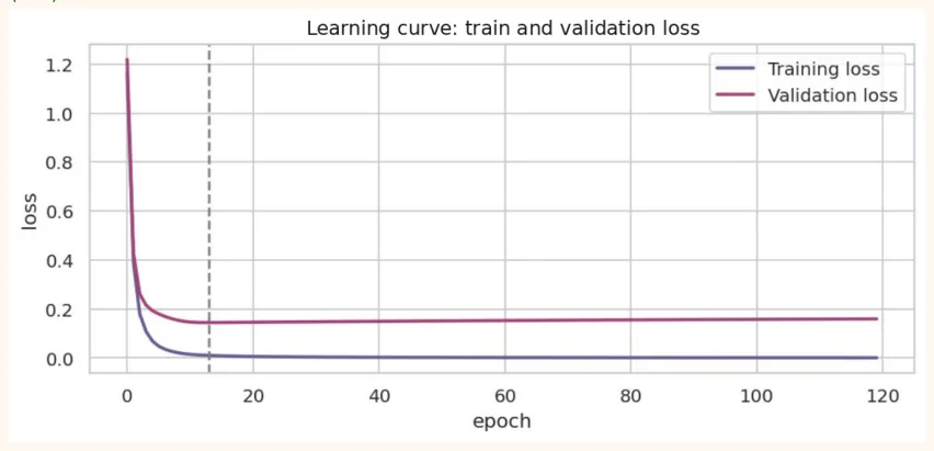
A neural network has a huge number of parameters, so it can memorize the training data. How to spot it: look at both the training loss and the validation loss at every epoch . If the training loss keeps falling but the validation loss starts going up , overfitting has begun.
OUTPUT (chart)
22.3 Regularization: the cure for overfitting
1) L2 Regularization (Weight Decay)
Remember Ridge from Chapter 13: adding a penalty on the squares of the weights to the loss. The same in a neural network: large weights are punished, so the network stays simple . In sklearn the parameter is alpha , in Keras it is kernel_regularizer=regularizers.l2(0.001) .
2) Dropout
During training, at every step some neurons are randomly switched off (set to 0) (for example 30% or 50%). The network cannot rely on any single neuron, so every neuron learns strong features. Dropout is switched off during testing.
3) Early Stopping
When the validation loss stops improving (for some number of epochs), stop the training and take back the best weights. This is the simplest and most effective method.
es = MLPClassifier(hidden_layer_sizes=(128, 64), early_stopping=True, validation_fraction=0.15, n_iter_no_change=10, max_iter=500, random_state=0)
es.fit(X_tr_s, y_tr)
print("max_iter was 500, training stopped at:", es.n_iter_, "epochs")
print("Best validation score:", round(es.best_validation_score_, 3))
print("Test accuracy:", round(es.score(X_te_s, y_te), 3))
OUTPUT max_iter was 500, training stopped at: 31 epochs Best validation score: 0.975 Test accuracy: 0.971
4) The effect of L2 (alpha)
for a in [0.0001, 0.01, 0.1, 1, 3]:
    m = MLPClassifier(hidden_layer_sizes=(128, 64), alpha=a, max_iter=500, random_state=0).fit(X_tr_s, y_tr)
    print("alpha =", str(a).ljust(7), "train:", round(m.score(X_tr_s, y_tr), 3), "  test:", round(m.score(X_te_s, y_te), 3))
OUTPUT
alpha = 0.0001  train:
1.0   test:
0.98
alpha = 0.01    train:
1.0   test:
0.978
alpha = 0.1     train:
1.0   test:
0.984
alpha = 1       train:
1.0   test:
0.98
alpha = 3       train:
0.996   test:
0.976
GOLDEN RULE
-
First apply Early Stopping ; it always helps.
-
Then, if needed, try Dropout (0.2 to 0.5) or L2 .
-
The most effective cure is often more data or a smaller network .
22.4 Batch Normalization
In deep networks the scale of each layer's inputs keeps changing, which makes training hard. Batch Normalization brings each layer's output (on every mini-batch) to mean 0 and std 1 , and then applies two learned parameters ( gamma for scale, beta for shift). Result: training is faster and more stable .
np.random.seed(0)
batch = np.random.randn(32, 4) * [1, 10, 100, 0.1] + [5, -20, 300, 0]   # 4 features, very different scales
print("Before  mean:", batch.mean(axis=0).round(1))
print("Before  std :", batch.std(axis=0).round(1))
eps = 1e-5
normed = (batch - batch.mean(axis=0)) / np.sqrt(batch.var(axis=0) + eps)
print("After   mean:", normed.mean(axis=0).round(2))
print("After   std :", normed.std(axis=0).round(2))
OUTPUT Before mean: [ 5.1 -18.9 297.3 0. ] Before std : [ 1.2 11.1 80.8 0.1] After mean: [-0. -0. -0. 0.] After std : [1. 1. 1. 1.]
22.5 Weight Initialization
The starting value (initial value) of the weights is very important. If all are zero, all neurons learn the same thing (symmetry). If they are very large, the activations blow up, and if they are very small, the signal dies out . Two famous methods:
| Name | Formula (std) | Used with which activation |
|---|---|---|
| Xavier / Glorot | sqrt(2 / (fan_in + fan_out)) | Sigmoid, Tanh (Keras default) |
| He | sqrt(2 / fan_in) | ReLU |
np.random.seed(0)
def forward_std(init, layers=10, width=256):
    a = np.random.randn(1000, width)
    stds = []
    for _ in range(layers):
        fan_in = a.shape[1]
        if init == "small (0.01)":
            W = np.random.randn(fan_in, width) * 0.01
        elif init == "large (1.0)":
            W = np.random.randn(fan_in, width) * 1.0
        else:
            W = np.random.randn(fan_in, width) * np.sqrt(2 / fan_in)   # He
            a = np.maximum(0, a @ W)             # ReLU stds.append(a.std()) return stds
for init in ["small (0.01)", "large (1.0)", "He"]:
    s = forward_std(init)
    print(init.ljust(14), "layer 1:", format(s[0], ".4g").ljust(10), "layer 5:", format(s[4], ".4g").ljust(11), "layer 10:", format(s[9], ".4g"))
OUTPUT small (0.01) layer 1: 0.09312 layer 5: 1.614e-05 layer 10: 3.094e-10 large (1.0) layer 1: 9.325 layer 5: 1.601e+05 layer 10: 2.532e+10 He layer 1: 0.8284 layer 5: 0.7855 layer 10: 0.6848 With He initialization the size of the signal stays roughly the same at every layer , whereas on the wrong scale it either shrinks to nothing or blows up .
22.6 Vanishing and Exploding Gradients
In backprop the gradient gets multiplied at every layer. If every factor is smaller than 1, the gradient dies out as it travels backwards ( vanishing ), and if it is bigger it blows up ( exploding ). The derivative of sigmoid is at most 0.25 , so in deep sigmoid networks the first layers learn nothing at all.
sig = lambda z:
1 / (1 + np.exp(-z))
np.random.seed(1)
depth = 10
for name, act, dact in [
("Sigmoid", sig, lambda a: a * (1 - a)),
("ReLU",    lambda z: np.maximum(0, z), lambda a: (a > 0).astype(float)),
]:
h = np.random.randn(64, 100)
Ws, As = [], [h]
for _ in range(depth):
    W = np.random.randn(100, 100) * np.sqrt(2 / 100)
    h = act(h @ W)
    Ws.append(W)
    As.append(h)
    g = np.ones_like(h)              # gradient at the last
    layer = 1
    mags = []
    for W, a in zip(reversed(Ws), reversed(As[1:])):
        g = (g * dact(a)) @ W.T
        mags.append(np.abs(g).mean())
        mags = mags[::-1]
        print(name.ljust(8), "gradient size, first layer:", format(mags[0], ".2e"),
        "| last layer:", format(mags[-1], ".2e"))
OUTPUT
Sigmoid  gradient size, first layer: 6.70e-06 | last layer: 2.54e-01
ReLU     gradient size, first layer: 1.86e+00 | last layer: 8.29e-01
22.7 Optimizers: making the network learn faster and better
Gradient descent updates the weights with w = w - lr * gradient . There are several better forms of the same idea:
| Optimizer | Idea | Pros / Cons |
|---|---|---|
| SGD | A direct step along the gradient of each mini- batch | Simple; can be slow, depends heavily on the learning rate |
| SGD + Momentum | Also keep the "speed" of previous steps | Fast in valleys, less oscillation |
| RMSprop | Adjusts each parameter's learning rate by the size of its gradient | Good for parameters with very different scales |
| Adam | A blend of Momentum + RMSprop | The most popular default; often works well without tuning |
Comparing solvers in sklearn (on Digits)
import time
for solver, kw in [("sgd", {"learning_rate_init": 0.01, "momentum": 0}),
("sgd", {"learning_rate_init": 0.01, "momentum": 0.9,
"nesterovs_momentum": True}),
("adam", {"learning_rate_init": 0.001})]:
m = MLPClassifier(hidden_layer_sizes=(128, 64), solver=solver, max_iter=60, random_state=0, **kw)
import warnings
warnings.filterwarnings("ignore")
m.fit(X_tr_s, y_tr)
tag = solver + (" + momentum" if kw.get("momentum", 0) > 0 else " (plain)")
if solver == "sgd"
else "adam"
print(tag.ljust(15), "final train loss:", round(m.loss_, 4), " test acc:", round(m.score(X_te_s, y_te), 3))
OUTPUT sgd (plain) final train loss: 0.4275 test acc: 0.904 sgd + momentum final train loss: 0.0206 test acc: 0.971 adam final train loss: 0.0042 test acc: 0.978
22.8 Learning Rate and Scheduling
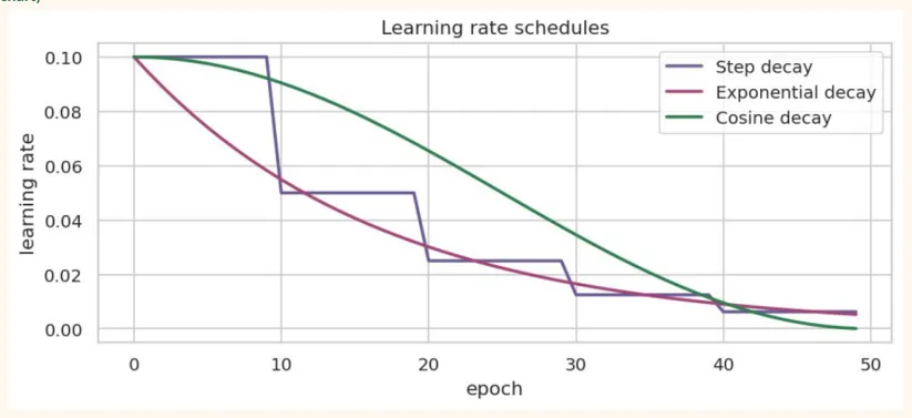
The learning rate (lr) is the most important hyperparameter. Too big: the loss jumps around or blows up. Too small: training is very slow. In scheduling we keep a big lr at the start (a fast journey) and then keep making it smaller (fine adjustment).
epochs = np.arange(0, 50)
lr0 = 0.1
step = lr0 * 0.5 ** (epochs // 10)           # halve every 10 epochs
expo = lr0 * np.exp(-0.06 * epochs)          # continuous exponential decrease
cosine = 0.5 * lr0 * (1 + np.cos(np.pi * epochs / 50))
print("epoch 0  :", lr0, round(expo[0], 4), round(cosine[0], 4))
print("epoch 25 : step", round(step[25], 4), " exp", round(expo[25], 4), " cosine",
round(cosine[25], 4))
print("epoch 49 : step", round(step[49], 4), " exp", round(expo[49], 4), " cosine",
round(cosine[49], 4))
fig, ax = plt.subplots(figsize=(9, 3.4))
ax.plot(epochs, step, color="#6B5B95", lw=2, label="Step decay")
ax.plot(epochs, expo, color="#A4457A", lw=2, label="Exponential decay")
ax.plot(epochs, cosine, color="#2F7D4F", lw=2, label="Cosine decay")
ax.set_xlabel("epoch")
ax.set_ylabel("learning rate")
ax.legend()
ax.set_title("Learning rate schedules")
plt.show()
OUTPUT
epoch 0 : 0.1 0.1 0.1 epoch 25 : step 0.025 exp 0.0223 cosine 0.05 epoch 49 : step 0.0062 exp 0.0053 cosine 0.0001 OUTPUT (chart)
22.9 All of this in Keras: a deep network and callbacks
Now we put everything into one Keras model: Dense + BatchNormalization + Dropout + L2 , the Adam optimizer, and callbacks ( EarlyStopping , ReduceLROnPlateau ). The multiclass labels are integers (0 to 9), so the loss is sparse_categorical_crossentropy .
from tensorflow import keras
from tensorflow.keras import layers, regularizers, callbacks
model = keras.Sequential([ keras.Input(shape=(64,)), layers.Dense(128, activation="relu", kernel_regularizer=regularizers.l2(1e-4)), layers.BatchNormalization(), layers.Dropout(0.3), layers.Dense(64, activation="relu"), layers.Dense(10, activation="softmax"), ])
model.compile(optimizer=keras.optimizers.Adam(learning_rate=0.001), loss="sparse_categorical_crossentropy", metrics=["accuracy"])
model.summary()
OUTPUT (sample) Model: "sequential" ┏━━━━━━━━━━━━━━━━━━━━━━━━━━━━━━━━━━━━━━━━━━┳━━━━━━━━━━━━━━━━━━━━━━━━━━┳━━━━━━━━━━━━━━━━━┓ ┃ ┃ ┃ ┃ Layer (type) Output Shape Param # ┡━━━━━━━━━━━━━━━━━━━━━━━━━━━━━━━━━━━━━━━━━━╇━━━━━━━━━━━━━━━━━━━━━━━━━━╇━━━━━━━━━━━━━━━━━┩ │ dense (Dense) │ (None, 128) │ 8,320 │ │ batch_normalization (BatchNormalization) │ (None, 128) │ 512 │ │ dropout (Dropout) │ (None, 128) │ 0 │ │ dense_1 (Dense) │ (None, 64) │ 8,256 │ │ dense_2 (Dense) │ (None, 10) │ 650 │ └──────────────────────────────────────────┴──────────────────────────┴─────────────────┘ Total params: 17,738 (69.29 KB) Trainable params: 17,482 (68.29 KB) Non-trainable params: 256 (1.00 KB)
22.10 Common Mistakes and Hands-on
Hands-on
-
Overfit it: run a (256,128) network on Digits with sgd and see for yourself the val loss going up in the learning curve.
-
Change alpha: change alpha from 0.0001 to 3 and write down the difference between train and test accuracy.
-
Optimizer race: change lr in the optimizer code above (what happens to SGD at 0.5?).
-
Dropout rate: try dropout 0.1, 0.3, 0.6 in the Keras model.
-
Callbacks: set patience to 3 and 20 and compare len(history.history["loss"]) .
KEY TAKEAWAYS
-
A deep network = more power but more risk of overfitting; start small.
-
How to spot overfitting: the train loss keeps falling while the validation loss goes up.
-
Regularization: Early Stopping (first choice), L2, Dropout; dropout in training, not in testing.
-
Batch Normalization normalizes the inputs of each layer, making training faster and more stable.
-
Initialization: He for ReLU, Xavier for sigmoid/tanh. Never zero initialization.
-
Vanishing gradient: the derivative of sigmoid is <= 0.25; ReLU and BatchNorm help.
-
Optimizers: SGD, Momentum, RMSprop, Adam. Adam (lr=0.001) is the usual default.
-
The learning rate is the most important hyperparameter; use scheduling and ReduceLROnPlateau.