Chapter 27: Autoencoders and Representation Learning
MODULE 5 | WEEK 27
Chapter 27: Autoencoders and Representation Learning
In the neural networks so far we were given the answer (label) . An Autoencoder is a network that learns on its own : it first compresses its input into a small summary (code) , and then tries to rebuild the original input from that summary. In this effort it learns the most important information in the data, and this is called Representation Learning . In this chapter we will see the structure of an autoencoder, the comparison with PCA , denoising , anomaly detection , and finally the idea of the VAE , which paves the way for the GAN of the next chapter.
27.1 What is an Autoencoder?
An autoencoder has three parts:
| Part | Job | Shape |
|---|---|---|
| Encoder | Compresses the input into a smallcode | Layers that keep reducing the size (64 -> 32 -> 8) |
| Bottleneck (Latent) | The smallest part; the summary of the information | A tiny layer (for example 8 numbers) |
| Decoder | Rebuilds the original input from the code | Layers that keep increasing the size (8 -> 32 - > 64) |
Input  ->  Encoder  ->  CODE (small)  ->  Decoder  ->  Reconstruction
 64                         8                         64
Loss = reconstruction error = mean( (Input - Reconstruction)^2 )
Target (y) = the Input itself!  (this is why it is also called "self-supervised")
27.2 Autoencoder vs PCA
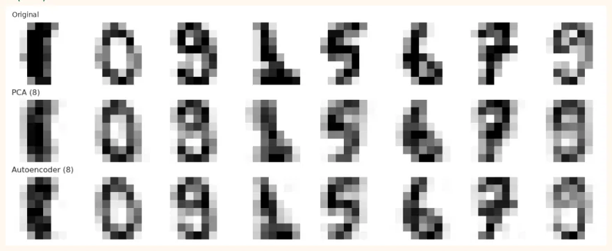
In Chapter 17 PCA also reduced 64 columns. PCA and the autoencoder have the same goal , but PCA compresses only in a linear (straight) way, whereas an autoencoder can also catch non-linear (curved) relationships. A comparison of compressing Digits down to 8 numbers with both:
import numpy as np
import matplotlib.pyplot as plt
import warnings
warnings.filterwarnings("ignore")
from sklearn.datasets import load_digits
from sklearn.model_selection import train_test_split
from sklearn.decomposition import PCA
from sklearn.neural_network import MLPRegressor
digits = load_digits()
X, y = digits.data / 16.0, digits.target                # 0 to 1
X_tr, X_te, y_tr, y_te = train_test_split(X, y, test_size=0.25,
random_state=42, stratify=y)
# PCA:
64 -> 8 -> 64
pca = PCA(n_components=8).fit(X_tr)
rec_pca = pca.inverse_transform(pca.transform(X_te))
# Autoencoder:
64 -> 64 -> 8 -> 64 -> 64   (target = the input itself)
ae = MLPRegressor(hidden_layer_sizes=(64, 8, 64), activation="relu", learning_rate_init=0.002, max_iter=3000, tol=1e-7, n_iter_no_change=100, random_state=0)
ae.fit(X_tr, X_tr)
rec_ae = ae.predict(X_te)
mse = lambda a, b:
np.mean((a - b) ** 2)
print("PCA (8 components)  reconstruction MSE:", round(mse(X_te, rec_pca), 4))
print("Autoencoder (8-d)   reconstruction MSE:", round(mse(X_te, rec_ae), 4))
print("Layer sizes of the autoencoder:", [ae.coefs_[0].shape[0]] + [c.shape[1] for c in ae.coefs_])
OUTPUT PCA (8 components) reconstruction MSE: 0.0245 Autoencoder (8-d) reconstruction MSE: 0.0186 Layer sizes of the autoencoder: [64, 64, 8, 64, 64] In this run the autoencoder's error came out lower than PCA's: even after compressing to 8 numbers it rebuilds the image better, because it can also learn curved relationships. (On small data and a small network the difference is not very big, and it can change a little from one seed to another.)
Looking at reconstructions
idx = np.arange(8)
fig, axes = plt.subplots(3, 8, figsize=(10, 4))
rows = [("Original", X_te), ("PCA (8)", rec_pca), ("Autoencoder (8)", rec_ae)]
for r, (name, data) in enumerate(rows):
    for c, i in enumerate(idx):
        axes[r, c].imshow(data[i].reshape(8, 8), cmap="gray_r", interpolation="nearest",
        vmin=0, vmax=1)
        axes[r, c].axis("off")
        axes[r, 0].set_title(name, fontsize=9, loc="left")
        plt.tight_layout()
        plt.show()
OUTPUT (chart)
27.3 Denoising Autoencoder
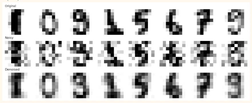
We deliberately add noise to the input and teach the network to rebuild the clean image. This way it learns to remove noise (cleaning old, blurry images, scanned papers).
rng = np.random.RandomState(0)
X_tr_noisy = np.clip(X_tr + rng.normal(0, 0.3, X_tr.shape), 0, 1)
X_te_noisy = np.clip(X_te + rng.normal(0, 0.3, X_te.shape), 0, 1)
dae = MLPRegressor(hidden_layer_sizes=(64, 16, 64), activation="relu",
learning_rate_init=0.003, max_iter=800, random_state=0)
dae.fit(X_tr_noisy, X_tr)                 # input:
noisy,  target:
CLEAN
denoised = dae.predict(X_te_noisy)
print("Error of the noisy image (vs the clean one):", round(mse(X_te_noisy, X_te), 4))
print("Error after denoising                      :", round(mse(denoised, X_te), 4))
fig, axes = plt.subplots(3, 8, figsize=(10, 4))
for r, (name, data) in enumerate([("Original", X_te), ("Noisy", X_te_noisy), ("Denoised", denoised)]):
    for c in range(8):
        axes[r, c].imshow(data[c].reshape(8, 8), cmap="gray_r", interpolation="nearest", vmin=0, vmax=1) axes[r, c].axis("off") axes[r, 0].set_title(name, fontsize=9, loc="left")
        plt.tight_layout()
        plt.show()
OUTPUT
Error of the noisy image (vs the clean one): 0.0527
Error after denoising                      : 0.0318
OUTPUT (chart)
27.4 Anomaly Detection: catching the odd one out
The idea: train the autoencoder on only "normal" data . It will rebuild normal things well , but it will rebuild an unusual (anomaly) thing badly , meaning its reconstruction error will be large . This is the method used to catch bank fraud, machine failure and network attacks.
The experiment: train the autoencoder on the digits 0 to 8 (never show it a 9), then see whether the error on a 9 in the test comes out higher.
from sklearn.metrics import roc_auc_score
normal = y_tr != 9
ae_n = MLPRegressor(hidden_layer_sizes=(64, 8, 64), activation="relu",
learning_rate_init=0.002, max_iter=3000,
tol=1e-7, n_iter_no_change=100, random_state=0)
ae_n.fit(X_tr[normal], X_tr[normal])             # only normal (without 9)
err = ((X_te - ae_n.predict(X_te)) ** 2).mean(axis=1)    # the error of each image
is_anomaly = (y_te == 9)
print("Mean error, normal images    :", round(err[~is_anomaly].mean(), 4))
print("Mean error, digit 9 (anomaly):", round(err[is_anomaly].mean(), 4))
print("ROC-AUC (spotting anomalies by error):", round(roc_auc_score(is_anomaly, err), 3))
fig, ax = plt.subplots(figsize=(8, 3.2))
ax.hist(err[~is_anomaly], bins=30, alpha=0.7, color="#6B5B95", label="Normal (0 to 8)")
ax.hist(err[is_anomaly], bins=30, alpha=0.7, color="#A4457A", label="Anomaly (9)")
ax.set_xlabel("reconstruction error")
ax.legend()
ax.set_title("Anomalies have a larger error")
plt.show()
OUTPUT Mean error, normal images : 0.0173 Mean error, digit 9 (anomaly): 0.0384 ROC-AUC (spotting anomalies by error): 0.891
OUTPUT (chart)
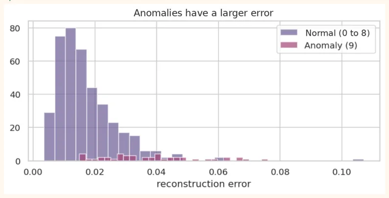
An AUC of 0.5 means guessing, 1.0 means perfect. Here the AUC is well above 0.5, which means spotting anomalies by error is possible (but not perfect, because 9 looks similar to digits like 4/7). To choose a threshold, pick on the validation data an error below which at least 95% of the normal cases stay.
27.5 Representation Learning: the features of the encoder
The encoder part of an autoencoder turns the data into 8 meaningful numbers . These numbers can be given as input to another model (such as a classifier). First the representation is learned without labels , and then we try to build a classifier even with few labels ( semi-supervised ).
from sklearn.linear_model import LogisticRegression
def encode(model, X):
    """Run the first two layers of the autoencoder (up to the bottleneck) by hand"""
    a = np.maximum(0, X @ model.coefs_[0] + model.intercepts_[0])
    return np.maximum(0, a @ model.coefs_[1] + model.intercepts_[1])
Z_tr, Z_te = encode(ae, X_tr), encode(ae, X_te)
print("Code shape:", Z_tr.shape, "(64 pixels -> 8 numbers)")
raw = LogisticRegression(max_iter=3000).fit(X_tr, y_tr)
code = LogisticRegression(max_iter=3000).fit(Z_tr, y_tr)
pca_f = LogisticRegression(max_iter=3000).fit(pca.transform(X_tr), y_tr)
print("Accuracy, original 64 pixels     :", round(raw.score(X_te, y_te), 3))
print("Accuracy, autoencoder's 8 numbers:", round(code.score(Z_te, y_te), 3))
print("Accuracy, PCA's 8 numbers        :", round(pca_f.score(pca.transform(X_te), y_te),
3))
OUTPUT
Code shape: (1347, 8) (64 pixels -> 8 numbers)
Accuracy, original 64 pixels     : 0.962
Accuracy, autoencoder's 8 numbers: 0.916
Accuracy, PCA's 8 numbers        : 0.9
Read carefully: even on just 8 numbers (an eighth of the original) the classifier gave nearly 92% accuracy , whereas on the original 64 pixels it was ~96%. The autoencoder's codes were better than PCA's 8 numbers . So most of the information survived in a representation 8 times smaller . This is representation learning : first learn
a meaningful summary of the data, then use it. Big models (BERT, GPT, Chapter 30) are much larger forms of this very idea.
# With few labels:
only 100 labelled images
small = np.random.RandomState(1).choice(len(X_tr), 100, replace=False)
raw100 = LogisticRegression(max_iter=3000).fit(X_tr[small], y_tr[small])
code100 = LogisticRegression(max_iter=3000).fit(Z_tr[small], y_tr[small])
print("Only 100 labels, original pixels   :", round(raw100.score(X_te, y_te), 3))
print("Only 100 labels, autoencoder codes:", round(code100.score(Z_te, y_te), 3))
OUTPUT Only 100 labels, original pixels : 0.902 Only 100 labels, autoencoder codes: 0.88
In this small experiment the original pixels did slightly better . This is why you should not assume that representation learning wins everywhere. The benefit shows up when there is a lot of unlabelled data and very little labelled data, and when the data is big and complex (images, text). Always keep a raw-features baseline alongside and look at the result yourself.
27.6 Autoencoders in Keras
Dense Autoencoder
from tensorflow import keras
from tensorflow.keras import layers
inputs = keras.Input(shape=(64,))
x = layers.Dense(32, activation="relu")(inputs)
code = layers.Dense(8, activation="relu", name="code")(x)      # bottleneck
x = layers.Dense(32, activation="relu")(code)
outputs = layers.Dense(64, activation="sigmoid")(x)            # pixels 0 to 1
autoencoder = keras.Model(inputs, outputs)
encoder = keras.Model(inputs, code)                            # just the encoder, separately
autoencoder.compile(optimizer="adam", loss="mse") autoencoder.summary() OUTPUT (sample)
Model: "functional"
┏━━━━━━━━━━━━━━━━━━━━━━━━━━━━━━━━━━━┳━━━━━━━━━━━━━━━━━━━━━━━━━━┳━━━━━━━━━━━━━━━━━┓
┃
┃
┃
┃
Layer (type) Output Shape Param #┡━━━━━━━━━━━━━━━━━━━━━━━━━━━━━━━━━━━╇━━━━━━━━━━━━━━━━━━━━━━━━━━╇━━━━━━━━━━━━━━━━━┩ |
|---|
│ input_layer (InputLayer) │ (None, 64) │ 0 │ |
│ dense (Dense) │ (None, 32) │ 2,080 │ |
│ code (Dense) │ (None, 8) │ 264 │ |
│ dense_1 (Dense) │ (None, 32) │ 288 │ |
│ dense_2 (Dense) │ (None, 64) │ 2,112 │└───────────────────────────────────┴──────────────────────────┴─────────────────┘ |
 Total params: 4,744 (18.53 KB)
 Trainable params: 4,744 (18.53 KB)
 Non-trainable params: 0 (0.00 B)
Convolutional Autoencoder (better for images)
On images, Conv2D + MaxPooling2D (encoder) and Conv2D + UpSampling2D (decoder) work better than Dense. UpSampling2D doubles the size of the image (the opposite of pooling).
def conv_p(k, in_ch, out_ch):
    return (k * k * in_ch + 1) * out_ch
layers_p = [conv_p(3, 1, 8), conv_p(3, 8, 4), conv_p(3, 4, 4), conv_p(3, 4, 8), conv_p(3, 8, 1)]
print("Parameters of each Conv2D:", layers_p)
print("Total:", sum(layers_p))
OUTPUT
Parameters of each Conv2D:
[80, 292, 148, 296, 73] Total:
889
inp = keras.Input(shape=(8, 8, 1))
x = layers.Conv2D(8, 3, padding="same", activation="relu")(inp)   # (8, 8, 8)
x = layers.MaxPooling2D(2)(x)                                      # (4, 4, 8)
x = layers.Conv2D(4, 3, padding="same", activation="relu")(x)      # (4, 4, 4)
x = layers.MaxPooling2D(2)(x)                                      # (2, 2, 4)  <- bottleneck:
16 numbers
x = layers.Conv2D(4, 3, padding="same", activation="relu")(x)      # (2, 2, 4)
x = layers.UpSampling2D(2)(x)                                      # (4, 4, 4)
x = layers.Conv2D(8, 3, padding="same", activation="relu")(x)      # (4, 4, 8)
x = layers.UpSampling2D(2)(x)                                      # (8, 8, 8)
out = layers.Conv2D(1, 3, padding="same", activation="sigmoid")(x) # (8, 8, 1)
conv_ae = keras.Model(inp, out)
conv_ae.compile(optimizer="adam", loss="mse")
print("Total parameters:", conv_ae.count_params())
OUTPUT (sample)
Total parameters: 889
27.7 Variational Autoencoder (VAE): the road to generation
The code of an ordinary autoencoder is a single list of numbers (a point) . In a VAE the encoder gives a distribution (mean and variance) instead of a point , and the code is a random sample from that distribution. This makes the latent space smooth , and by sampling new codes we can create new images from the decoder : in other words, a generative model out of an autoencoder.
Encoder ->  mu, log_var   (the 2 parts of a distribution)
            z = mu + sigma * epsilon,   epsilon ~ Normal(0, 1)    <- reparameterization
trick
Decoder ->  reconstruction
Loss = reconstruction loss  +  KL divergence(distribution, Normal(0,1))
       (make it accurate)        (keep the latent space tidy)
np.random.seed(0)
mu, log_var = np.array([1.0, -0.5]), np.array([-1.0, 0.0])       # outputs of the encoder (2-d
latent)
sigma = np.exp(0.5 * log_var)
samples = []
for _ in range(5):
    eps = np.random.randn(2)           # random noise
    z = mu + sigma * eps               # reparameterization trick samples.append(z)
    print("5 different latent samples from the same input:")
    print(np.array(samples).round(2))
    kl = -0.5 * np.sum(1 + log_var - mu**2 - np.exp(log_var))
    print("KL divergence:", round(kl, 3))
OUTPUT
5 different latent samples
from the same input:
[[ 2.07 -0.1 ] [ 1.59  1.74] [ 2.13 -1.48] [ 1.58 -0.65] [ 0.94 -0.09]] KL divergence:
0.809
The purpose of the reparameterization trick : by writing the random sampling as mu + sigma * epsilon , the gradient can reach mu and sigma (backprop can run), because the randomness is only in epsilon .
27.8 Common Mistakes and Hands-on
Hands-on
-
Change the bottleneck: set the bottleneck of the NumPy/sklearn autoencoder to 2, 4, 8, 16 and plot the reconstruction MSE.
-
Change the noise: try noise std 0.1, 0.3, 0.6 in denoising.
-
Anomaly: make 0 the anomaly instead of 9 and look at the AUC.
-
Compare with PCA: write the MSE of PCA and the autoencoder in a table for every bottleneck size.
-
Keras: in Colab, build a Dense autoencoder (784 -> 64 -> 784) on fashion_mnist and look at the reconstruction chart.
KEY TAKEAWAYS
-
Autoencoder = Encoder + Bottleneck + Decoder; the target is the input itself (self-supervised).
-
Keep the bottleneck small, otherwise the network just copies.
-
PCA is linear compression, an autoencoder is non-linear; an autoencoder often gives a smaller error.
-
Denoising AE: noisy input, clean target.
-
Anomaly detection: train on normal data only; the anomaly's reconstruction error is large.
-
Representation learning: the small codes of the encoder can be given as input to other models; the benefit depends on the data and the problem, so always keep a raw baseline alongside.
-
A Conv autoencoder (Conv2D + UpSampling2D) is better for images.
-
VAE: the code is a distribution; sampling and generation are possible through the reparameterization trick.