Chapter 23: Convolutional Neural Networks (CNN)
MODULE 5 | WEEK 23
Chapter 23: Convolutional Neural Networks (CNN)
For images, an ordinary (Dense) network is very weak. The Convolutional Neural Network (CNN) is designed especially for images, and today it powers everything from face recognition, reading X-rays and self-driving cars to the camera in your phone. In this chapter we will see what convolution, filter, stride, padding and pooling are, what the structure of a CNN looks like, how to count parameters, and how to build a CNN in Keras.
23.1 What is image data?
For a computer an image is a grid of numbers . Each number is the brightness of one pixel . A greyscale image has one channel (0 = black, a big number = white). A color (RGB) image has 3 channels (Red, Green, Blue). So the shape of an image is (height, width, channels) .
import numpy as np
from sklearn.datasets import load_digits
digits = load_digits()
img = digits.images[3]               # one image
print("Shape      :", img.shape, "(height, width) greyscale")
print("Min / Max  :", img.min(), "/", img.max())
print("Label      :", digits.target[3])
print(img.astype(int))
OUTPUT Shape : (8, 8) (height, width) greyscale Min / Max : 0.0 / 15.0 Label : 3 [[ 0 0 7 15 13 1 0 0] [ 0 8 13 6 15 4 0 0] [ 0 2 1 13 13 0 0 0] [ 0 0 2 15 11 1 0 0] [ 0 0 0 1 12 12 1 0] [ 0 0 0 0 1 10 8 0] [ 0 0 8 4 5 14 9 0] [ 0 0 7 13 13 9 0 0]]
In Chapter 8 we looked at Digits. A color image (such as a 224x224 photo) has 224 x 224 x 3 = 150,528 numbers.
| Image | Shape (H, W, C) | Total numbers |
|---|---|---|
| Digits (our dataset) | (8, 8, 1) | 64 |
| MNIST handwritten digits | (28, 28, 1) | 784 |
| CIFAR-10 small color image | (32, 32, 3) | 3,072 |
| An ordinary photo | (224, 224, 3) | 150,528 |
23.2 Why is a Dense network not enough for images?
If we feed a 224x224x3 image straight into a Dense layer (after flattening) and keep just 1000 neurons, the weights of the first layer alone come to 150,528 x 1000 = more than 150 million . A second reason: a Dense network loses the sense of position , because it turns the pixels into one long queue, whereas the relationship between neighboring pixels is the most important thing in images.
pixels = 224 * 224 * 3
print("Input numbers:", pixels)
print("Weights + bias of Dense(1000):", pixels * 1000 + 1000)
print("Weights + bias of Conv2D(32 filters, 3x3):", 3 * 3 * 3 * 32 + 32)
OUTPUT Input numbers: 150528 Weights + bias of Dense(1000): 150529000 Weights + bias of Conv2D(32 filters, 3x3): 896 The CNN's answer: small filters slide over the whole image and use the same weights again and again ( weight sharing ). This gives far fewer parameters.
23.3 Convolution: a filter sliding over the image
A filter (kernel) is a small grid of numbers (for example 3x3). We place it on top of the image, multiply the numbers in the same positions and add them up ; this makes one output pixel . Then the filter moves forward one step ( stride ). The new image that is formed by sliding over the whole image is called a feature map .
ANALOGY
A torch that lights up a small spot. You sweep the torch across the whole wall and ask "is there a straight line here? is there a corner here?". The filter is that torch, and each filter looks for one particular thing (a vertical line, a horizontal line, a corner).
def conv2d(image, kernel, stride=1, padding=0):
    if padding > 0:
        image = np.pad(image, padding)          # zeros at the edges
        kh, kw = kernel.shape
        out_h = (image.shape[0] - kh) // stride + 1
        out_w = (image.shape[1] - kw) // stride + 1
        out = np.zeros((out_h, out_w))
        for i in range(out_h):
            for j in range(out_w):
                patch = image[i*stride:i*stride+kh, j*stride:j*stride+kw] out[i, j] = np.sum(patch * kernel)
            return out
small = np.array([[1, 2, 0, 1], [0, 1, 3, 1], [2, 1, 0, 0], [1, 0, 1, 2]], dtype=float)
kernel = np.array([[1, 0], [0, -1]], dtype=float)
print(conv2d(small, kernel))
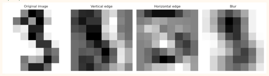
OUTPUT [[ 0. -1. -1.] [-1. 1. 3.] [ 2. 0. -2.]] Check by hand: multiply the top-left 2x2 part [[1,2],[0,1]] with the filter [[1,0],[0,-1]] : 11 + 20 + 00 + 1(-1) = 0 , and the first output number came out as 0. Now real filters ( edge detectors ) on a Digits image:
import matplotlib.pyplot as plt
img = digits.images[3] / 16.0
vertical   = np.array([[-1, 0, 1], [-2, 0, 2], [-1, 0, 1]], dtype=float)   # vertical lines
horizontal = vertical.T                                                    # horizontal lines
blur       = np.ones((3, 3)) / 9                                           # blur
maps = {"Original image": img, "Vertical edge": conv2d(img, vertical, padding=1), "Horizontal edge": conv2d(img, horizontal, padding=1), "Blur": conv2d(img, blur, padding=1)}
fig, axes = plt.subplots(1, 4, figsize=(10, 2.8))
for ax, (name, m) in zip(axes, maps.items()):
    ax.imshow(m, cmap="gray_r", interpolation="nearest")
    ax.set_title(name, fontsize=9)
    ax.axis("off")
    plt.tight_layout()
    plt.show()
OUTPUT (chart)
23.4 Stride, Padding and Output Size
Stride: how many pixels the filter moves at a time (1 or 2). A bigger stride = a smaller output. Padding: putting zeros around the edges of the image. valid padding = no zeros (the output gets smaller). same padding = just enough zeros so that the output has the same size as the input (at stride 1).
Output size = floor( (N + 2P - F) / S ) + 1
N = input size
F = filter size
P = padding
S = stride
def out_size(N, F, P=0, S=1):
return (N + 2 * P - F) // S + 1
print("8x8, 3x3 filter, valid (P=0), S=1 :", out_size(8, 3, 0, 1))
print("8x8, 3x3 filter, same  (P=1), S=1 :", out_size(8, 3, 1, 1))
print("8x8, 3x3 filter, P=0, S=2         :", out_size(8, 3, 0, 2))
print("28x28, 5x5 filter, P=0, S=1       :", out_size(28, 5, 0, 1))
print("224x224, 7x7 filter, P=3, S=2     :", out_size(224, 7, 3, 2))
OUTPUT 8x8, 3x3 filter, valid (P=0), S=1 : 6 8x8, 3x3 filter, same (P=1), S=1 : 8 8x8, 3x3 filter, P=0, S=2 : 3 28x28, 5x5 filter, P=0, S=1 : 24 224x224, 7x7 filter, P=3, S=2 : 112
23.5 ReLU and Pooling
After convolution we apply ReLU (turn negative values into 0). Then Pooling makes the image smaller so that there is less computation and the network is not bothered by small shifts (for example a digit moved slightly to one side). Max Pooling keeps the largest number from each region.
def max_pool(fmap, size=2):
    h, w = fmap.shape[0] // size, fmap.shape[1] // size
    out = np.zeros((h, w))
    for i in range(h):
        for j in range(w):
            out[i, j] = fmap[i*size:(i+1)*size, j*size:(j+1)*size].max()
        return out
fmap = np.array([[1, 3, 2, 1], [4, 6, 5, 0], [7, 2, 9, 8], [1, 0, 3, 4]], dtype=float)
print("Feature map:\n", fmap)
print("Max pool 2x2:\n", max_pool(fmap))
print("Average pool 2x2:\n", fmap.reshape(2, 2, 2, 2).mean(axis=(1, 3)))
OUTPUT Feature map: [[1. 3. 2. 1.] [4. 6. 5. 0.] [7. 2. 9. 8.] [1. 0. 3. 4.]] Max pool 2x2: [[6. 5.] [7. 9.]] Average pool 2x2: [[3.5 2. ] <u>[2.5 6. ]]</u> ANALOGY
Making a list of the top scorers of the 4 sections of a class: from each section, pick only the student with the highest marks . The information has shrunk but the most important thing is still there. Max pooling also keeps the strongest signal of every region.
23.6 The complete structure of a CNN
A typical CNN is a repeating pattern : [Conv -> ReLU -> Pool] several times, then Flatten , then Dense layers, and finally softmax/sigmoid .
Image -> [Conv+ReLU -> Pool] -> [Conv+ReLU -> Pool] -> Flatten -> Dense -> Softmax
  First part: FEATURE EXTRACTION (extracting features from the image)
  Second part: CLASSIFICATION (a decision from the features)
In the early layers the image keeps getting smaller (because of Pool) but the channels (filters) keep increasing (16, 32, 64...). So we shrink the size of the image and pack more kinds of features into it.
Counting parameters
Conv2D parameters = (filter_h x filter_w x input_channels + 1) x filters
Dense parameters  = (inputs + 1) x neurons
Pooling, Flatten, Dropout = 0 parameters
def conv_params(fh, fw, in_ch, filters): return (fh * fw * in_ch + 1) * filters
def dense_params(inputs, neurons):          return (inputs + 1) * neurons
c1 = conv_params(3, 3, 1, 16)      # 16 filters on Digits (8,8,1)
c2 = conv_params(3, 3, 16, 32)     # 32 filters
d1 = dense_params(2 * 2 * 32, 64)  # 128 numbers after Flatten
d2 = dense_params(64, 10)
print("Conv2D(16, 3x3) :", c1)
print("Conv2D(32, 3x3) :", c2)
print("Dense(64)       :", d1)
print("Dense(10)       :", d2)
print("Total CNN       :", c1 + c2 + d1 + d2)
print("Comparison: a Dense-only network 64->128->64->10:", dense_params(64, 128) + dense_params(128, 64) + dense_params(64, 10))
OUTPUT
Conv2D(16, 3x3) : 160
Conv2D(32, 3x3) : 4640
Dense(64)       : 8256
Dense(10)       : 650
Total CNN       : 13706
Comparison: a Dense-only network 64->128->64->10: 17226
23.7 Preparing the data for a CNN
A CNN needs input of shape (samples, height, width, channels) . The Digits images are 2D, so we have to add a channel axis. We scale the pixels between 0 and 1 (dividing by 16).
from sklearn.model_selection import train_test_split
X = digits.images / 16.0                 # (1797, 8, 8), 0 to 1
y = digits.target
X = X[..., np.newaxis]                   # (1797, 8, 8, 1)  channel axis
print("CNN input shape:", X.shape)
X_tr, X_te, y_tr, y_te = train_test_split(X, y, test_size=0.25, random_state=42, stratify=y)
print("Train:", X_tr.shape, " Test:", X_te.shape)
print("Pixel range:", X_tr.min(), "to", X_tr.max())
OUTPUT CNN input shape: (1797, 8, 8, 1) Train: (1347, 8, 8, 1) Test: (450, 8, 8, 1) Pixel range: 0.0 to 1.0
23.8 CNN in Keras
from tensorflow import keras
from tensorflow.keras import layers
cnn = keras.Sequential([ keras.Input(shape=(8, 8, 1)), layers.Conv2D(16, (3, 3), padding="same", activation="relu"), layers.MaxPooling2D((2, 2)), layers.Conv2D(32, (3, 3), padding="same", activation="relu"), layers.MaxPooling2D((2, 2)), layers.Flatten(), layers.Dense(64, activation="relu"), layers.Dense(10, activation="softmax"), ])
cnn.compile(optimizer="adam", loss="sparse_categorical_crossentropy", metrics=["accuracy"])
cnn.summary()
OUTPUT (sample) Model: "sequential"
┏━━━━━━━━━━━━━━━━━━━━━━━━━━━━━━━━━━━┳━━━━━━━━━━━━━━━━━━━━━━━━━━┳━━━━━━━━━━━━━━━━━┓
┃
┃
┃
┃
 Layer (type)                       Output Shape                      Param #
┡━━━━━━━━━━━━━━━━━━━━━━━━━━━━━━━━━━━╇━━━━━━━━━━━━━━━━━━━━━━━━━━╇━━━━━━━━━━━━━━━━━┩
│ conv2d (Conv2D)                   │ (None, 8, 8, 16)         │             160 │
│ max_pooling2d (MaxPooling2D)      │ (None, 4, 4, 16)         │               0 │
│ conv2d_1 (Conv2D)                 │ (None, 4, 4, 32)         │           4,640 │
│ max_pooling2d_1 (MaxPooling2D)    │ (None, 2, 2, 32)         │               0 │
│ flatten (Flatten)                 │ (None, 128)              │               0 │
│ dense (Dense)                     │ (None, 64)               │           8,256 │
│ dense_1 (Dense)                   │ (None, 10)               │             650 │
└───────────────────────────────────┴──────────────────────────┴─────────────────┘
 Total params: 13,706 (53.54 KB)
 Trainable params: 13,706 (53.54 KB)
 Non-trainable params: 0 (0.00 B)
23.9 Data Augmentation
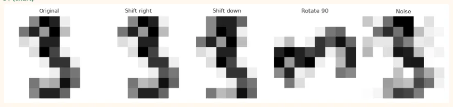
A CNN needs a lot of images. When data is scarce, Data Augmentation makes new images from the same image by changing it slightly (shift, rotate, zoom, flip). The network feels there is more data, and it overfits less .
fig, axes = plt.subplots(1, 5, figsize=(10, 2.2))
im = digits.images[3]
variants = {"Original": im, "Shift right": np.roll(im, 1, axis=1), "Shift down": np.roll(im, 1, axis=0), "Rotate 90": np.rot90(im), "Noise": np.clip(im + np.random.RandomState(0).randn(8, 8) * 2, 0, 16)}
for ax, (name, v) in zip(axes, variants.items()):
    ax.imshow(v, cmap="gray_r", interpolation="nearest")
    ax.set_title(name, fontsize=9)
    ax.axis("off")
    plt.tight_layout()
    plt.show()
OUTPUT (chart)
KEEP IN MIND
Choose augmentation to suit the purpose . If you rotate the digit 6 by 180 degrees it becomes a 9 , so big rotations are wrong on digits. Flipping a picture of a cat (horizontal flip) is fine.
augment = keras.Sequential([
layers.RandomTranslation(0.1, 0.1),   # shift up to 10%
layers.RandomRotation(0.05),          # rotate slightly
layers.RandomZoom(0.1),
])
aug_cnn = keras.Sequential([
keras.Input(shape=(8, 8, 1)),
augment,                              # runs only during training
layers.Conv2D(16, 3, padding="same", activation="relu"),
layers.MaxPooling2D(),
layers.Flatten(),
layers.Dense(10, activation="softmax"),
]) Augmentation layers are active only during training ; in predict / evaluate they switch themselves off, so they have no effect on the test data.
23.10 Common Mistakes and Hands-on
Hands-on
-
Conv by hand: run the 3x3 filter [[0,1,0],[1,-4,1],[0,1,0]] on some Digits image with the conv2d function and make a chart.
-
Output size: using the formula, find the size after a 3x3 conv (valid) on 28x28 followed by a 2x2 pool.
-
Parameters: count the parameters of a Conv2D(64, 3x3) that runs on 32 channels yourself, and check them against model.summary() .
-
Change the filters: change 16/32 in the CNN to 8/16 and 32/64; write down the comparison of accuracy and parameters.
-
Your own images: load keras.datasets.fashion_mnist in Colab, build a CNN (28x28x1) and make a confusion matrix.
KEY TAKEAWAYS
-
An image = a grid of numbers, shape (H, W, C). Greyscale has 1 channel, RGB has 3 channels.
-
Convolution: a small filter slides over the image and makes a feature map. Weights are shared, hence fewer parameters.
-
Output size = floor((N + 2P - F) / S) + 1. same padding keeps the size unchanged.
-
ReLU brings in non-linearity; Max Pooling reduces the size and protects against small shifts.
-
CNN = [Conv-ReLU-Pool] x several times, then Flatten and a Dense classifier.
-
Conv params = (fh x fw x in_ch + 1) x filters. Pool/Flatten/Dropout have 0 parameters.
-
On small data, reduce overfitting with Data Augmentation and Dropout.