Chapter 24: Advanced CNN Architectures and Image Projects
MODULE 5 | WEEK 24
Chapter 24: Advanced CNN Architectures and Image Projects
In the last chapter you built a small CNN. Over the past 25 years researchers have made CNNs much better: LeNet, AlexNet, VGG, Inception, ResNet, MobileNet, EfficientNet . In this chapter we will understand their basic ideas (such as the skip connection , 1x1 convolution and depthwise separable convolution ), and then learn the most useful thing of all: Transfer Learning , that is, using big models trained by others for your own problem. At the end we will see the method of a complete image classification project .
24.1 The journey of CNN architectures
Each new architecture solved one particular problem . Below is a short sketch of the famous models (parameters are approximate counts):
| Model | Year | Key idea | Approx. parameters |
|---|---|---|---|
| LeNet-5 | 1998 | The first successful CNN (handwritten digits, bank cheques) | 60 thousand |
| AlexNet | 2012 | ReLU, Dropout, training on GPU; won ImageNet and started the deep learning era | 61 million |
| VGG-16 | 2014 | Stacking only 3x3 filters very deep (simple but heavy) | 138 million |
| Inception (GoogLeNet) | 2014 | Filters of several sizes in one layer, and 1x1 convolution | 7 million |
| ResNet-50 | 2015 | Skip (residual) connection: very deep networks became trainable | 25.6 million |
| MobileNetV2 | 2018 | Depthwise separable convolution: lightweight for phones | 3.5 million |
| EfficientNet-B0 | 2019 | Growing depth, width and resolution together in a balanced way | 5.3 million |
24.2 The problem of deep networks and ResNet
In Chapter 22 we saw the vanishing gradient. The strange thing was that in very deep networks even the training accuracy started to drop (the degradation problem ), meaning the network could not learn at all. ResNet's answer: in every block, also send the input x straight ahead and add it to the output of the block:
Plain block :   output = F(x)
Residual block:   output = F(x) + x        <-- skip(shortcut) connection
Residual Block: Keras Functional API
Sequential is not enough for a skip connection, because the data travels along two paths. For this there is the Functional API : apply each layer to its input like a function.
from tensorflow import keras
from tensorflow.keras import layers
def residual_block(x, filters):
    shortcut = x
    x = layers.Conv2D(filters, 3, padding="same", activation="relu")(x)
    x = layers.Conv2D(filters, 3, padding="same")(x)
    x = layers.Add()([x, shortcut])          # F(x) + x
    return layers.Activation("relu")(x)
inputs = keras.Input(shape=(8, 8, 16))
outputs = residual_block(inputs, 16)
block = keras.Model(inputs, outputs)
print("Parameters of the block:", block.count_params())
OUTPUT (sample) Parameters of the block: 4640
24.3 1x1 Convolution and the idea of Inception
A 1x1 convolution only mixes the channels at each pixel (it does not change the spatial size). With it the channels can be reduced or increased and a lot of computation is saved. Inception used it as a bottleneck : first reduce the channels with a 1x1, then apply the expensive 3x3 conv.
def conv_params(k, in_ch, out_ch):
    return (k * k * in_ch + 1) * out_ch
direct = conv_params(3, 256, 256)
bottleneck = conv_params(1, 256, 64) + conv_params(3, 64, 64) + conv_params(1, 64, 256)
print("Direct 3x3 conv (256 -> 256)            :", direct)
print("Bottleneck (1x1 -> 3x3 -> 1x1)          :", bottleneck)
print("Savings:", round(100 * (1 - bottleneck / direct), 1), "%")
OUTPUT Direct 3x3 conv (256 -> 256) : 590080 Bottleneck (1x1 -> 3x3 -> 1x1) : 70016 Savings: 88.1 % ResNet-50 is built on exactly this bottleneck block , which is why in spite of having 50 layers it has only 25.6 million parameters, while VGG-16 has 138 million.
24.4 Depthwise Separable Convolution (MobileNet)
An ordinary convolution runs over all the input channels for every filter. MobileNet breaks it into two light parts:
-
Depthwise: a separate 3x3 filter of its own on each input channel (the channels do not mix with each other).
-
Pointwise: a 1x1 conv that mixes the channels.
in_ch, out_ch, k = 128, 128, 3
standard = (k * k * in_ch + 1) * out_ch
depthwise = k * k * in_ch + in_ch                  # each channel's own 3x3 filter + bias pointwise = (1 * 1 * in_ch + 1) * out_ch separable = depthwise + pointwise print("Standard 3x3 conv (128 -> 128)  :", standard) print("Depthwise + Pointwise           :", separable, "(", depthwise, "+", pointwise, ")") print("How many times fewer:", round(standard / separable, 1), "x")
OUTPUT Standard 3x3 conv (128 -> 128) : 147584 Depthwise + Pointwise : 17792 ( 1280 + 16512 ) How many times fewer: 8.3 x Roughly 8 times fewer parameters and computation, at the cost of a small loss of accuracy. This is why MobileNet runs on phones and small devices.
24.5 Global Average Pooling vs Flatten
Older networks (VGG) had Flatten + big Dense layers , which held a very large share of the parameters. Newer networks use Global Average Pooling (GAP) : it takes the whole average of each feature map and turns it into a single number.
# Output of the last conv layer: 7 x 7 pixels, 512 channels
h, w, c, classes = 7, 7, 512, 10
flatten_head = (h * w * c + 1) * 256 + (256 + 1) * classes     # Flatten -> Dense(256) ->
Dense(10)
gap_head = (c + 1) * classes                                    # GAP -> Dense(10)
print("Numbers after Flatten    :", h * w * c)
print("Numbers after GAP        :", c)
print("Parameters of Flatten head:", flatten_head)
print("Parameters of GAP head    :", gap_head)
OUTPUT
Numbers after Flatten    : 25088
Numbers after GAP        : 512
Parameters of Flatten head: 6425354
Parameters of GAP head    : 5130
GAP gives far fewer parameters , lowers the risk of overfitting, and the network can run on an image of any size .
24.6 Transfer Learning
A network trained on big data like ImageNet (14 million images, 1000 categories) has already learned lines, edges and textures in its first layers and things like eyes, wheels and leaves in its deeper layers. We use that same learned knowledge on our own small data.
KEEP IN MIND
-
Fine-tuning always comes after feature extraction , and with a very small learning rate . A big lr spoils the pre-trained weights.
-
You must compile again whenever trainable has been changed.
-
weights="imagenet" needs the internet to download (it usually works in Colab).
24.7 Image Project: the workflow
Whatever the problem, the skeleton of an image classification project stays the same. We will look at it in a practical way on Digits (which runs without the internet), and then apply the same steps to Fashion-MNIST and to data in your own folders.
-
Understand the data: shape, classes, the count of each class, look at some images.
-
Split + scale: train/test, pixels from 0 to 1.
-
Baseline: a simple model (like Logistic Regression).
-
Model: a CNN or Transfer Learning.
-
Evaluate: accuracy, confusion matrix, classification report.
-
Error analysis: where does the model make mistakes? Look at the wrong images.
-
Save + a predict function.
import matplotlib.pyplot as plt
from sklearn.datasets import load_digits
from sklearn.model_selection import train_test_split
from sklearn.preprocessing import StandardScaler
from sklearn.neural_network import MLPClassifier
from sklearn.metrics import confusion_matrix, classification_report
digits = load_digits()
X, y, imgs = digits.data / 16.0, digits.target, digits.images
X_tr, X_te, y_tr, y_te, im_tr, im_te = train_test_split(
X, y, imgs, test_size=0.25, random_state=42, stratify=y)
print("Count of each class:", np.bincount(y))
model = MLPClassifier(hidden_layer_sizes=(128, 64), max_iter=400, random_state=0)
model.fit(X_tr, y_tr)
pred = model.predict(X_te)
print("Test accuracy:", round((pred == y_te).mean(), 3))
print()
print(classification_report(y_te, pred, digits=3))
OUTPUT
Count of each class: [178 182 177 183 181 182 181 179 174 180]
Test accuracy: 0.987
precision recall f1-score support |
|---|
0 1.000 0.978 0.989 45 |
1 0.957 0.978 0.968 46 |
2 1.000 1.000 1.000 44 |
3 1.000 1.000 1.000 46 |
4 0.978 1.000 0.989 45 |
5 1.000 0.978 0.989 46 |
6 1.000 0.978 0.989 45 |
7 1.000 1.000 1.000 45 |
8 0.953 0.953 0.953 43 |
9 0.978 1.000 0.989 45 |
accuracy 0.987 450 |
macro avg 0.987 0.987 0.987 450 |
weighted avg 0.987 0.987 0.987 450 |
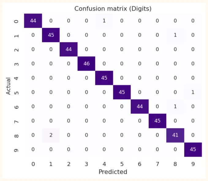
The confusion matrix tells us which two classes the model confuses :
import seaborn as sns
cm = confusion_matrix(y_te, pred)
fig, ax = plt.subplots(figsize=(6.2, 5))
sns.heatmap(cm, annot=True, fmt="d", cmap="Purples", cbar=False, ax=ax)
ax.set_xlabel("Predicted")
ax.set_ylabel("Actual")
ax.set_title("Confusion matrix (Digits)")
plt.show()
errors = np.where(pred != y_te)[0]
print("Wrong predictions:", len(errors), "/", len(y_te))
OUTPUT Wrong predictions: 6 / 450 OUTPUT (chart)
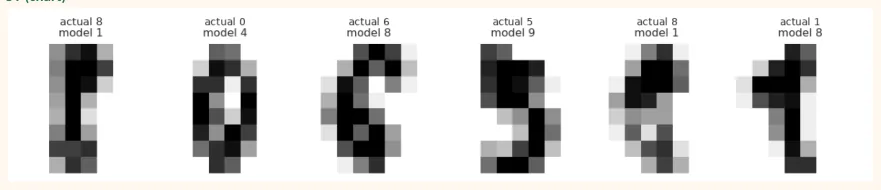
Error analysis: look at the wrongly predicted images yourself. Often the reason is clearly visible (bad handwriting, two similar-looking digits):
n = min(8, len(errors))
fig, axes = plt.subplots(1, n, figsize=(10, 1.9))
for ax, idx in zip(np.atleast_1d(axes), errors[:n]):
    ax.imshow(im_te[idx], cmap="gray_r", interpolation="nearest")
    ax.set_title("actual %d\nmodel %d" % (y_te[idx], pred[idx]), fontsize=9)
    ax.axis("off")
    plt.tight_layout()
    plt.show()
OUTPUT (chart)
After this, save the model. In Keras there is the .keras format, and next we wrap it in a predict function :
model.save("digits_cnn.keras")                    # Keras model
loaded = keras.models.load_model("digits_cnn.keras")
def predict_digit(img_8x8):
    x = (img_8x8 / 16.0).reshape(1, 8, 8, 1)       # the same preprocessing as in training
    probs = loaded.predict(x, verbose=0)[0]
    return int(probs.argmax()), float(probs.max())
24.8 Fashion-MNIST: a complete Keras image project (Colab)
Fashion-MNIST : 28x28 greyscale images of 70,000 pieces of clothing, in 10 categories (60,000 train, 10,000 test). Keras downloads this data itself, so run it in Colab .
from tensorflow import keras
from tensorflow.keras import layers
import numpy as np
(X_train, y_train), (X_test, y_test) = keras.datasets.fashion_mnist.load_data()
print(X_train.shape, y_train.shape, X_test.shape)
class_names = ["T-shirt/top", "Trouser", "Pullover", "Dress", "Coat",
"Sandal", "Shirt", "Sneaker", "Bag", "Ankle boot"]
X_train = X_train[..., np.newaxis] / 255.0     # (60000, 28, 28, 1), 0 to 1
X_test  = X_test[..., np.newaxis] / 255.0
print(X_train.shape, X_train.max())
OUTPUT (sample)
(60000, 28, 28) (60000,) (10000, 28, 28) (60000, 28, 28, 1) 1.0
model = keras.Sequential([ keras.Input(shape=(28, 28, 1)), layers.Conv2D(32, 3, activation="relu"), layers.MaxPooling2D(), layers.Conv2D(64, 3, activation="relu"),
layers.MaxPooling2D(), layers.Flatten(), layers.Dropout(0.3), layers.Dense(10, activation="softmax"), ]) model.compile(optimizer="adam", loss="sparse_categorical_crossentropy", metrics=["accuracy"]) model.summary() OUTPUT (sample) Model: "sequential"
┏━━━━━━━━━━━━━━━━━━━━━━━━━━━━━━━━━━━┳━━━━━━━━━━━━━━━━━━━━━━━━━━┳━━━━━━━━━━━━━━━━━┓
┃
┃
┃
┃
 Layer (type)                       Output Shape                      Param #
┡━━━━━━━━━━━━━━━━━━━━━━━━━━━━━━━━━━━╇━━━━━━━━━━━━━━━━━━━━━━━━━━╇━━━━━━━━━━━━━━━━━┩
│ conv2d (Conv2D)                   │ (None, 26, 26, 32)       │             320 │
│ max_pooling2d (MaxPooling2D)      │ (None, 13, 13, 32)       │               0 │
│ conv2d_1 (Conv2D)                 │ (None, 11, 11, 64)       │          18,496 │
│ max_pooling2d_1 (MaxPooling2D)    │ (None, 5, 5, 64)         │               0 │
│ flatten (Flatten)                 │ (None, 1600)             │               0 │
│ dropout (Dropout)                 │ (None, 1600)             │               0 │
│ dense (Dense)                     │ (None, 10)               │          16,010 │
└───────────────────────────────────┴──────────────────────────┴─────────────────┘
 Total params: 34,826 (136.04 KB)
 Trainable params: 34,826 (136.04 KB)
 Non-trainable params: 0 (0.00 B)
24.9 Loading images from your own folders
In a real project the images are in folders , one folder per class. Keras can load them directly:
dataset/
  train/
    cat/  img1.jpg  img2.jpg ...
    dog/  img1.jpg ...
  val/
    cat/ ...
    dog/ ...
train_ds = keras.utils.image_dataset_from_directory(
    "dataset/train", image_size=(160, 160), batch_size=32)
val_ds = keras.utils.image_dataset_from_directory(
    "dataset/val", image_size=(160, 160), batch_size=32)
print(train_ds.class_names)        # folder names = classes
train_ds = train_ds.prefetch(buffer_size=tf.data.AUTOTUNE)   # fast loading (import
tensorflow as tf)
In Colab turn on the GPU : Runtime > Change runtime type > GPU . CNN training is very slow on a CPU.
24.10 Common Mistakes and Hands-on
Hands-on
-
Counting parameters: work out the parameters of Conv2D(64, 3x3) running on 32 channels and of its depthwise separable version, and compare them.
-
ResNet block: with the Functional API build a small network with 2 residual blocks and look at model.summary() .
-
Transfer Learning: in Colab, put 30 images each of 3 classes (for example chai, biryani, burger) in folders and build a classifier with MobileNetV2.
-
Fashion-MNIST: run the CNN above, make a confusion matrix and say which two classes are confused the most.
-
Fine-tuning: after feature extraction, unfreeze the last 30 layers and see whether the accuracy improves or not.
KEY TAKEAWAYS
-
From LeNet to EfficientNet, each architecture solved one problem: depth (ResNet), less computation (Inception, MobileNet).
-
The skip connection F(x) + x carries the gradient straight back, which lets networks of 50-100+ layers train.
-
1x1 convolution and depthwise separable convolution cut parameters and computation a lot.
-
Global Average Pooling has fewer parameters than Flatten + big Dense, and reduces overfitting.
-
Transfer Learning: freeze the pre-trained base, train a new head; then fine-tune with a small lr if needed.
-
The skeleton of an image project: data, baseline, model, evaluation, confusion matrix, error analysis, save and predict.
-
Always keep the preprocessing of training and prediction the same.