Chapter 21: Neural Network Fundamentals aur Backpropagation
MODULE 5 | WEEK 21
Chapter 21: Neural Network Fundamentals aur Backpropagation
Ab hum Deep Learning ki duniya me qadam rakhte hain. Module 4 me tumne dekha ke model data se seekhta hai; ab dekhenge ke neural network insani dimagh se prerit hokar kaise seekhta hai, uske andar neuron, layer, activation, loss kya hote hain, aur sab se aham: network apni galti se backpropagation ke zariye kaise seekhta hai. Pehle sab kuch NumPy se hath se banayenge taake jadoo samajh aaye, phir TensorFlow/Keras me wohi kaam chand lines me karenge.
21.1 Deep Learning aur Neural Network kya hai?
Neural Network ek aisa model hai jo bohat se chhote chhote neurons (hisaab karne wali ikaiyon) ko layers me jod kar banta hai. Jab layers bohat zyada hon ( deep ), to isay Deep Learning kehte hain. Chapter 1 ki chhatri yaad karo: AI > Machine Learning > Deep Learning .
21.2 Ek neuron: sab se chhoti ikai
Ek neuron ye 3 kaam karta hai: (1) har input ko apne weight se guna karta hai, (2) sab ko jama kar ke bias add karta hai, (3) nateeje ko activation function se guzarta hai.
z = w1*x1 + w2*x2 + ... + wn*xn + b      (weighted sum)
a = activation(z)                           (neuron ka output)
21.3 Activation Functions
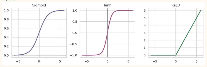
Agar activation na ho to chahe kitni bhi layers laga lo, poora network sirf ek seedhi lakeer (linear) ban kar reh jata hai. Activation function network me non-linearity (tedhapan) lata hai, jis se wo pecheeda patterns seekh sakta hai.
| Activation | Formula (mukhtasar) | Output range | Kahan istemal hota hai |
|---|---|---|---|
| Sigmoid | 1 / (1 + e^-z) | 0 se 1 | Binary classification ka aakhri layer |
| Tanh | (e^z - e^-z) / (e^z + e^-z) | -1 se 1 | Purane hidden layers, RNN ke andar |
| ReLU | max(0, z) | 0 se infinity | Hidden layers ka default |
| Softmax | e^zi / jama(e^zj) | 0 se 1 (jama = 1) | Multiclass classification ka aakhri layer |
import numpy as np
import matplotlib.pyplot as plt
z = np.linspace(-6, 6, 200)
funcs = {
"Sigmoid": 1 / (1 + np.exp(-z)),
"Tanh": np.tanh(z),
"ReLU": np.maximum(0, z),
}
colors = ["#6B5B95", "#A4457A", "#2F7D4F"]
fig, axes = plt.subplots(1, 3, figsize=(10, 3.2))
for ax, (name, y), c in zip(axes, funcs.items(), colors):
    ax.plot(z, y, color=c, lw=2.5)
    ax.axhline(0, color="gray", lw=0.8)
    ax.axvline(0, color="gray", lw=0.8)
    ax.set_title(name)
    plt.tight_layout()
    plt.show()
OUTPUT (chart)
Softmax ek list of numbers (scores) ko probabilities me badalta hai jin ka jama hamesha 1 hota hai:
def softmax(scores):
    e = np.exp(scores - np.max(scores))   # stability ke liye max ghatao
    return e / e.sum()
scores = np.array([2.0, 1.0, 0.1])         # 3 classes ke raw scores
p = softmax(scores)
print("Probabilities:", p.round(3))
print("Jama:", p.sum().round(3))
print("Predicted class:", p.argmax())
OUTPUT
Probabilities: [0.659 0.242 0.099]
Jama: 1.0
Predicted class: 0
SUNEHRA USOOL
-
Hidden layers me pehli pasand ReLU (tez aur simple).
-
Binary output: aakhri layer me sigmoid (1 neuron).
-
Multiclass output: aakhri layer me softmax (har class ka 1 neuron).
-
Regression output: aakhri layer me koi activation nahi (linear).
21.4 Layers aur Forward Propagation
Network me neurons layers me hote hain: Input layer (data lene wali), ek ya zyada Hidden layers (andar ki soch), aur Output layer (nateeja). Data input se output ki taraf jata hai, isay Forward Propagation kehte hain. Poori layer ka hisaab matrix multiplication se hota hai.
Layer ka hisaab:   A = activation( X @ W + b )
X : (samples, input_features)
W : (input_features, neurons)
b : (neurons,)
A : (samples, neurons)
np.random.seed(0)
X = np.random.randn(5, 4)          # 5 samples, 4 features
W1 = np.random.randn(4, 3) * 0.5   # hidden layer: 3 neurons
b1 = np.zeros(3)
W2 = np.random.randn(3, 1) * 0.5   # output layer: 1 neuron
b2 = np.zeros(1)
relu = lambda z: np.maximum(0, z)
sigmoid = lambda z: 1 / (1 + np.exp(-z))
H = relu(X @ W1 + b1)              # hidden layer ka output
out = sigmoid(H @ W2 + b2)         # final probability
print("X shape  :", X.shape)
print("H shape  :", H.shape)
print("out shape:", out.shape)
print("Probabilities:", out.ravel().round(3))
print("Parameters:", W1.size + b1.size + W2.size + b2.size)
OUTPUT
X shape  : (5, 4)
H shape  : (5, 3)
out shape: (5, 1)
Probabilities: [0.2   0.405 0.269 0.382 0.423]
Parameters: 19
21.5 Loss Function: network ki galti ka paimana
Loss batata hai ke network ki prediction sach se kitni door hai. Training ka maqsad is loss ko kam se kam karna hai (Chapter 13 ka cost function yaad karo).
| Masla | Loss | Aakhri layer |
|---|---|---|
| Regression | MSE (Mean Squared Error) | 1 neuron, koi activation nahi |
| Binary classification | Binary Cross-Entropy | 1 neuron, sigmoid |
| Multiclass (labels 0,1,2...) | Sparse Categorical Cross-Entropy | N neurons, softmax |
| Multiclass (one-hot labels) | Categorical Cross-Entropy | N neurons, softmax |
y_true = np.array([1, 0, 1, 1])
y_pred = np.array([0.9, 0.2, 0.6, 0.3])   # network ki probabilities
mse = np.mean((y_true - y_pred) ** 2)
bce = -np.mean(y_true * np.log(y_pred) + (1 - y_true) * np.log(1 - y_pred))
print("MSE:", round(mse, 4))
print("Binary Cross-Entropy:", round(bce, 4))
# Agar network bohat yaqeen se ghalat ho to cross-entropy bohat barh jati hai
print("Sahi aur yaqeen (0.99):", round(-np.log(0.99), 3))
print("Ghalat aur yaqeen (0.01):", round(-np.log(0.01), 3))
OUTPUT
MSE: 0.175
Binary Cross-Entropy: 0.5108
Sahi aur yaqeen (0.99): 0.01
Ghalat aur yaqeen (0.01): 4.605
Cross-entropy ghalat aur pur-yaqeen prediction ko bohat sakht saza deti hai, isi liye classification me MSE ke bajaye ye behtar hai.
21.6 Backpropagation: network kaise seekhta hai
Forward propagation se prediction aati hai aur loss nikalta hai. Ab sawal ye hai: kaun sa weight kitna zimmedar hai is galti ka? Backpropagation loss se shuru kar ke peeche ki taraf chalta hai aur chain rule se har weight ka gradient (loss me tabdeeli ki raftar) nikalta hai. Phir Gradient Descent (Chapter 13) weights ko thora sa theek karta hai.
Chain rule: ek chhota hath se hisaab
Sab se saada network: 1 input x, 1 weight w, 1 bias b, sigmoid, aur squared loss.
z = w*x + b
a = sigmoid(z)
L = (a - y)^2
Chain rule:
dL/dw = dL/da  *  da/dz  *  dz/dw
dL/da = 2*(a - y)
da/dz = a*(1 - a)          (sigmoid ka derivative)
dz/dw = x
x, y = 2.0, 1.0
w, b = 0.5, 0.0
# Forward
z = w * x + b
a = 1 / (1 + np.exp(-z))
L = (a - y) ** 2
# Backward (chain rule)
dL_da = 2 * (a - y)
da_dz = a * (1 - a)
dz_dw = x
dL_dw = dL_da * da_dz * dz_dw
# Numerical check:
w ko zara sa hila kar loss dekho
eps = 1e-6
a2 = 1 / (1 + np.exp(-((w + eps) * x + b)))
numeric = ((a2 - y) ** 2 - L) / eps
print("Loss:", round(L, 5))
print("Chain rule gradient :", round(dL_dw, 5))
print("Numerical gradient  :", round(numeric, 5))
OUTPUT Loss: 0.07233 Chain rule gradient : -0.21151 Numerical gradient : -0.21151
Dono gradient barabar aaye, yani backprop ka hisaab sahi hai. Is tareeqe ko gradient checking kehte hain aur ye debugging me kaam aata hai.
21.7 NumPy me poora chhota Neural Network (zero se)
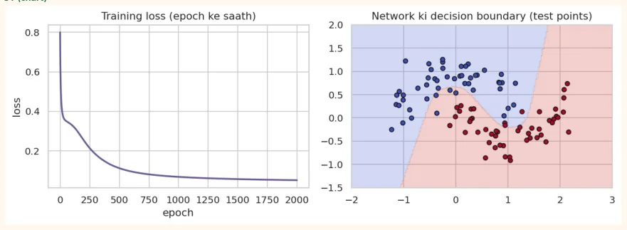
Ab hum upar ke sab hisse jod kar ek 2-layer network banate hain jo make_moons (do tedhe chand) ka masla hal karega, jo seedhi lakeer se hal nahi hota.
from sklearn.datasets import make_moons
from sklearn.model_selection import train_test_split
X, y = make_moons(n_samples=400, noise=0.2, random_state=42)
X_train, X_test, y_train, y_test = train_test_split(
X, y, test_size=0.25, random_state=42, stratify=y)
y_tr = y_train.reshape(-1, 1)
print("Train:", X_train.shape, " Test:", X_test.shape)
OUTPUT
Train: (300, 2)  Test: (100, 2)
np.random.seed(1)
n_hidden, lr, epochs = 8, 0.5, 2000
W1 = np.random.randn(2, n_hidden) * 0.5
b1 = np.zeros((1, n_hidden))
W2 = np.random.randn(n_hidden, 1) * 0.5
b2 = np.zeros((1, 1))
sigmoid = lambda z: 1 / (1 + np.exp(-z))
losses = []
for epoch in range(epochs):
    # ---- Forward ----
    Z1 = X_train @ W1 + b1
    A1 = np.tanh(Z1)
    Z2 = A1 @ W2 + b2
    A2 = sigmoid(Z2)
    loss = -np.mean(y_tr * np.log(A2 + 1e-9) + (1 - y_tr) * np.log(1 - A2 + 1e-9))
    losses.append(loss)
    # ---- Backward ----
    m = len(X_train)
    dZ2 = (A2 - y_tr) / m                 # sigmoid + cross-entropy ka saaf gradient
    dW2 = A1.T @ dZ2
    db2 = dZ2.sum(axis=0, keepdims=True)
    dZ1 = (dZ2 @ W2.T) * (1 - A1 ** 2)    # tanh ka derivative
    dW1 = X_train.T @ dZ1
    db1 = dZ1.sum(axis=0, keepdims=True)
    # ---- Update ----
    W1 -= lr * dW1; b1 -= lr * db1
    W2 -= lr * dW2; b2 -= lr * db2
    if epoch % 400 == 0:
        print("epoch", epoch, " loss:", round(loss, 4))
def predict(X):
    return (sigmoid(np.tanh(X @ W1 + b1) @ W2 + b2) > 0.5).astype(int).ravel()
print("Train accuracy:", round((predict(X_train) == y_train).mean(), 3))
print("Test accuracy :", round((predict(X_test) == y_test).mean(), 3))
OUTPUT
epoch 0  loss: 0.8005
epoch 400  loss: 0.139
epoch 800  loss: 0.0778
epoch 1200  loss: 0.0626
epoch 1600  loss: 0.0557
Train accuracy: 0.977
Test accuracy : 0.93
Loss curve aur network ki seekhi hui decision boundary dekhte hain:
fig, axes = plt.subplots(1, 2, figsize=(10, 3.6))
axes[0].plot(losses, color="#6B5B95", lw=2)
axes[0].set_title("Training loss (epoch ke saath)")
axes[0].set_xlabel("epoch")
axes[0].set_ylabel("loss")
xx, yy = np.meshgrid(np.linspace(-2, 3, 200), np.linspace(-1.5, 2, 200))
grid = np.c_[xx.ravel(), yy.ravel()]
axes[1].contourf(xx, yy, predict(grid).reshape(xx.shape), alpha=0.25, cmap="coolwarm")
axes[1].scatter(X_test[:, 0], X_test[:, 1], c=y_test, cmap="coolwarm", edgecolor="k", s=25)
axes[1].set_title("Network ki decision boundary (test points)")
plt.tight_layout()
plt.show()
OUTPUT (chart)
21.8 TensorFlow aur Keras ka taruf
Hath se backprop likhna samajhne ke liye acha hai, magar asli kaam me hum TensorFlow use karte hain. TensorFlow Google ki deep learning library hai, aur Keras uska aasan interface (tf.keras) hai. Ye khud gradient nikalta hai ( automatic differentiation ), GPU par chalta hai, aur bade models sambhalta hai.
Keras ka 5-step tareeqa
-
Model banao:
keras.Sequential([...])me layers ki list. -
Compile karo: optimizer, loss aur metrics batao.
-
Fit karo:
model.fit(X, y, epochs=..., validation_split=...)se training. -
Evaluate karo:
model.evaluate(X_test, y_test). -
Predict karo:
model.predict(X_new).
from tensorflow import keras
from tensorflow.keras import layers
model = keras.Sequential([
keras.Input(shape=(2,)),
layers.Dense(8, activation="relu"),     # hidden layer: 8 neurons
layers.Dense(1, activation="sigmoid"),  # output: probability
])
model.compile(optimizer="adam",
loss="binary_crossentropy",
metrics=["accuracy"])
model.summary()
OUTPUT (namoona)
Model: "sequential"
┏━━━━━━━━━━━━━━━━━━━━━━━━━━━━━━━━━━━┳━━━━━━━━━━━━━━━━━━━━━━━━━━┳━━━━━━━━━━━━━━━━━┓
┃ Layer (type)                       Output Shape                      Param # ┃┃┃
┡━━━━━━━━━━━━━━━━━━━━━━━━━━━━━━━━━━━╇━━━━━━━━━━━━━━━━━━━━━━━━━━╇━━━━━━━━━━━━━━━━━┩
│ dense (Dense)                     │ (None, 8)                │              24 │
│ dense_1 (Dense)                   │ (None, 1)                │               9 │
└───────────────────────────────────┴──────────────────────────┴─────────────────┘
 Total params: 33 (132.00 B)
 Trainable params: 33 (132.00 B)
 Non-trainable params: 0 (0.00 B)
YAAD RAKHO
Param # ka hisaab: pehli Dense: 2 inputs x 8 neurons + 8 bias = 24 . Doosri: 8 x 1 + 1 = 9 . Kul 33 . None ka matlab batch size koi bhi ho sakta hai.
history = model.fit(X_train, y_train,
epochs=100, batch_size=32,
validation_split=0.2, verbose=0)
test_loss, test_acc = model.evaluate(X_test, y_test, verbose=0)
print("Test accuracy:", round(test_acc, 3))
print("Pehli 5 probabilities:", model.predict(X_test[:5], verbose=0).ravel().round(2))
print("Asli labels          :", y_test[:5])
OUTPUT (namoona)
Test accuracy: 0.950
Pehli 5 probabilities: [0.88 0.26 0.22 0.14 0.06]
Asli labels          : [1 0 0 0 0]
Dhyan do: epoch ka matlab poore training data par ek poora chakkar , batch_size=32 ka matlab har update 32 samples dekh kar hota hai, aur validation_split=0.2 training data ka 20% validation ke liye alag rakhta hai taake overfitting pakdi ja sake (Chapter 12).
Neural network ko sklearn ke MLPClassifier se bhi chala sakte hain (ye bhi asli neural network hai), jis se tum Colab ke baghair bhi apne laptop par seekh sakti ho:
from sklearn.neural_network import MLPClassifier
mlp = MLPClassifier(hidden_layer_sizes=(8,), activation="relu",
max_iter=2000, random_state=1)
mlp.fit(X_train, y_train)
print("sklearn MLP test accuracy:", round(mlp.score(X_test, y_test), 3))
print("Layers ke weights ki shapes:", [w.shape for w in mlp.coefs_])
OUTPUT
sklearn MLP test accuracy: 0.95
Layers ke weights ki shapes: [(2, 8), (8, 1)]
21.9 Aam Galtiyan aur Hands-on
AAM GALTIYAN
-
Input scale na karna. Neural networks ko scaled data (StandardScaler ya 0 se 1) chahiye, warna training dheemi ya ghalat hoti hai.
-
Aakhri layer ka activation/loss ghalat chunna (jaise multiclass me sigmoid ya binary me softmax ke saath galat loss).
-
Shapes ka ghalat hona:
(None, 2)input par 3 features dena. -
Sirf train accuracy dekhna. Hamesha validation/test bhi dekho.
-
Learning rate bohat bara (loss uchhalta hai) ya bohat chhota (seekhta hi nahi).
Hands-on
-
Neurons badlo: NumPy network me
n_hiddenko 2, 4, 16 karo aur decision boundary ka farq dekho. -
Activation badlo: hidden layer me tanh ki jagah ReLU lagao (derivative: z>0 par 1, warna 0).
-
Learning rate:
lrko 0.01, 0.5, 5 karo aur loss curve ka muqabla karo. -
Dataset badlo:
make_circlespar wohi network chalao. -
Keras me:
Dense(8)koDense(32)karo aurmodel.summary()me Param # ka hisaab khud verify karo.
KEY TAKEAWAYS
-
Neuron = weighted sum + bias + activation. Weights aur bias hi seekhe jate hain.
-
Hidden layers me ReLU; binary me sigmoid; multiclass me softmax; regression me linear output.
-
Loss network ki galti napta hai: regression me MSE, classification me cross-entropy.
-
Backpropagation = chain rule se har weight ka gradient; phir gradient descent se update.
-
Keras ke 5 steps: Sequential, compile, fit, evaluate, predict.
model.summary()se parameters check karo. -
Neural network table wale chhote data par aksar Random Forest se behtar nahi hota; uski taqat images, text aur sequences me hai.