Chapter 24: CNN ki Advanced Architectures aur Image Projects
MODULE 5 | WEEK 24
Chapter 24: CNN ki Advanced Architectures aur Image Projects
Pichle chapter me tumne ek chhota CNN banaya. Pichle 25 saalon me researchers ne CNN ko bohat behtar banaya: LeNet, AlexNet, VGG, Inception, ResNet, MobileNet, EfficientNet . Is chapter me un ke bunyadi idea (jaise skip connection , 1x1 convolution , depthwise separable convolution ) samjhenge, phir sab se kaam ki cheez seekhenge: Transfer Learning , yani dusron ke train kiye hue bade models ko apne masle ke liye istemal karna. Aakhir me ek mukammal image classification project ka tareeqa dekhenge.
24.1 CNN architectures ka safar
Har nayi architecture ne ek khaas masla hal kiya. Neeche mashhoor models ka mukhtasar khaka hai (parameters qareeb ki ginti me):
| Model | Saal | Khaas idea | Taqreeban parameters |
|---|---|---|---|
| LeNet-5 | 1998 | Pehla kamyab CNN (haath se likhe number, bank cheques) | 60 hazaar |
| AlexNet | 2012 | ReLU, Dropout, GPU par training; ImageNet jeeta aur deep learning ka daur shuru kiya | 61 million |
| VGG-16 | 2014 | Sirf 3x3 filters ko bohat gehra stack karna (saada magar bhari) | 138 million |
| Inception (GoogLeNet) | 2014 | Ek layer me kai size ke filters aur 1x1 convolution | 7 million |
| ResNet-50 | 2015 | Skip (residual) connection: bohat gehre network train hone lage | 25.6 million |
| MobileNetV2 | 2018 | Depthwise separable convolution: phone ke liye halka | 3.5 million |
| EfficientNet-B0 | 2019 | Depth, width aur resolution ko ek sath balance se barhana | 5.3 million |
24.2 Gehre network ka masla aur ResNet
Chapter 22 me hum ne vanishing gradient dekha. Ajeeb baat ye thi ke bohat gehre network ki training accuracy bhi kam hone lagti thi ( degradation problem ), yani wo seekh hi nahi pata tha. ResNet ka jawab: har block me input x ko seedha agay bhi bhej do aur block ke output me jama kar do:
Plain block :   output = F(x)
Residual block:   output = F(x) + x        <-- skip (shortcut) connection
OUTPUT
Plain    network: pehli layer ka gradient = 3.32e-65
Residual network: pehli layer ka gradient = 2.61e+00
Plain network me gradient pehli layer tak bilkul mar gaya (e-65), jab ke residual me wo sehatmand size me pohancha. Isi liye ResNet 50, 101 ya 152 layers tak train ho sakta hai.
Residual Block: Keras Functional API
Skip connection ke liye Sequential kaafi nahi, kyun ke data do raaston par jata hai. Iske liye Functional API hai: har layer ko function ki tarah input par lagao.
from tensorflow import keras
from tensorflow.keras import layers
def residual_block(x, filters):
    shortcut = x
    x = layers.Conv2D(filters, 3, padding="same", activation="relu")(x)
    x = layers.Conv2D(filters, 3, padding="same")(x)
    x = layers.Add()([x, shortcut])          # F(x) + x
    return layers.Activation("relu")(x)
inputs = keras.Input(shape=(8, 8, 16))
outputs = residual_block(inputs, 16)
block = keras.Model(inputs, outputs)
print("Block ke parameters:", block.count_params())
OUTPUT (namoona)
Block ke parameters: 4640
24.3 1x1 Convolution aur Inception ka idea
1x1 convolution har pixel par sirf channels ko milata hai (spatial size nahi badalta). Isse channels kam ya zyada kiye ja sakte hain aur computation bohat bachta hai. Inception ne ise bottleneck ki tarah istemal kiya: pehle 1x1 se channels ghatao, phir mehnga 3x3 conv lagao.
def conv_params(k, in_ch, out_ch):
    return (k * k * in_ch + 1) * out_ch
direct = conv_params(3, 256, 256)
bottleneck = conv_params(1, 256, 64) + conv_params(3, 64, 64) + conv_params(1, 64, 256)
print("Seedha 3x3 conv (256 -> 256)            :", direct)
print("Bottleneck (1x1 -> 3x3 -> 1x1)          :", bottleneck)
print("Bachat:", round(100 * (1 - bottleneck / direct), 1), "%")
OUTPUT
Seedha 3x3 conv (256 -> 256)            : 590080
Bottleneck (1x1 -> 3x3 -> 1x1)          : 70016
Bachat: 88.1 %
ResNet-50 isi bottleneck block par bana hai, is liye 50 layers hone ke bawajood sirf 25.6 million parameters hain, jab ke VGG-16 ke 138 million.
24.4 Depthwise Separable Convolution (MobileNet)
Aam convolution har filter ke liye sab input channels par chalta hai. MobileNet isko do halke hisson me tod deta hai:
-
Depthwise: har input channel par alag apna 3x3 filter (channels aapas me nahi milte).
-
Pointwise: ek 1x1 conv jo channels ko milata hai.
in_ch, out_ch, k = 128, 128, 3
standard = (k * k * in_ch + 1) * out_ch
depthwise = k * k * in_ch + in_ch                  # har channel ka apna 3x3 filter + bias
pointwise = (1 * 1 * in_ch + 1) * out_ch
separable = depthwise + pointwise
print("Aam 3x3 conv (128 -> 128)       :", standard)
print("Depthwise + Pointwise           :", separable, "(", depthwise, "+", pointwise, ")")
print("Kitna kam:", round(standard / separable, 1), "guna")
OUTPUT
Aam 3x3 conv (128 -> 128)       : 147584
Depthwise + Pointwise           : 17792 ( 1280 + 16512 )
Kitna kam: 8.3 guna
Taqreeban 8 guna kam parameters aur computation, thori si accuracy ki qurbani ke saath. Isi wajah se MobileNet phone aur chhote devices par chalta hai.
24.5 Global Average Pooling vs Flatten
Purane networks (VGG) me Flatten + bari Dense layers hoti thi, jin me parameters ka bohat bara hissa hota tha. Naye networks Global Average Pooling (GAP) istemal karte hain: har feature map ka poora average le kar ek hi number bana deta hai.
# Aakhri conv layer ka output: 7 x 7 pixels, 512 channels
h, w, c, classes = 7, 7, 512, 10
flatten_head = (h * w * c + 1) * 256 + (256 + 1) * classes     # Flatten -> Dense(256) ->
Dense(10)
gap_head = (c + 1) * classes                                    # GAP -> Dense(10)
print("Flatten ke baad numbers  :", h * w * c)
print("GAP ke baad numbers      :", c)
print("Flatten wale head ke parameters:", flatten_head)
print("GAP wale head ke parameters    :", gap_head)
OUTPUT
Flatten ke baad numbers  : 25088
GAP ke baad numbers      : 512
Flatten wale head ke parameters: 6425354
GAP wale head ke parameters    : 5130
GAP se parameters bohat kam hote hain, overfitting ka khatra kam hota hai, aur network kisi bhi tasveer ke size par chal sakta hai.
24.6 Transfer Learning
ImageNet jaise bade data (14 million tasveerein, 1000 qismein) par train hue network ne pehli layers me lakeerein, kinare, texture aur gehri layers me aankhein, pahiye, patton jaisi cheezein pehle se seekh li hoti hain. Hum wohi seekha hua ilm apne chhote data par istemal karte hain.
OUTPUT (namoona)
Base output shape : (None, 5, 5, 1280)
Trainable parameters: 6405
DHYAN RAKHO
-
Fine-tuning hamesha feature extraction ke baad , aur bohat chhote learning rate se. Bara lr pre-trained weights ko bigad deta hai.
-
Compile dobara karna zaroori hai jab
trainablebadla ho. -
weights="imagenet"download ke liye internet chahiye (Colab me aam taur par chalta hai).
24.7 Image Project: tareeqa-e-kaar
Chahe masla kuch bhi ho, image classification project ka dhancha wohi rehta hai. Hum ise Digits par (jo bina internet ke chal jata hai) practical tareeqe se dekhte hain, phir wohi qadam Fashion-MNIST aur apne folder wale data par lagayenge.
-
Data samjho: shape, classes, har class ki ginti, kuch tasveerein dekho.
-
Split + scale: train/test, pixels ko 0 se 1.
-
Baseline: koi saada model (jaise Logistic Regression).
-
Model: CNN ya Transfer Learning.
-
Evaluate: accuracy, confusion matrix, classification report.
-
Error analysis: model kahan ghalti karta hai? Ghalat tasveerein dekho.
-
Save + predict function.
import matplotlib.pyplot as plt
from sklearn.datasets import load_digits
from sklearn.model_selection import train_test_split
from sklearn.preprocessing import StandardScaler
from sklearn.neural_network import MLPClassifier
from sklearn.metrics import confusion_matrix, classification_report
digits = load_digits()
X, y, imgs = digits.data / 16.0, digits.target, digits.images
X_tr, X_te, y_tr, y_te, im_tr, im_te = train_test_split(
X, y, imgs, test_size=0.25, random_state=42, stratify=y)
print("Har class ki ginti:", np.bincount(y))
model = MLPClassifier(hidden_layer_sizes=(128, 64), max_iter=400, random_state=0)
model.fit(X_tr, y_tr)
pred = model.predict(X_te)
print("Test accuracy:", round((pred == y_te).mean(), 3))
print()
print(classification_report(y_te, pred, digits=3))
OUTPUT
Har class ki ginti: [178 182 177 183 181 182 181 179 174 180]
Test accuracy: 0.987
precision recall f1-score support |
|---|
0 1.000 0.978 0.989 45 |
1 0.957 0.978 0.968 46 |
2 1.000 1.000 1.000 44 |
3 1.000 1.000 1.000 46 |
4 0.978 1.000 0.989 45 |
5 1.000 0.978 0.989 46 |
6 1.000 0.978 0.989 45 |
7 1.000 1.000 1.000 45 |
8 0.953 0.953 0.953 43 |
9 0.978 1.000 0.989 45 |
accuracy 0.987 450 |
macro avg 0.987 0.987 0.987 450 |
weighted avg 0.987 0.987 0.987 450 |
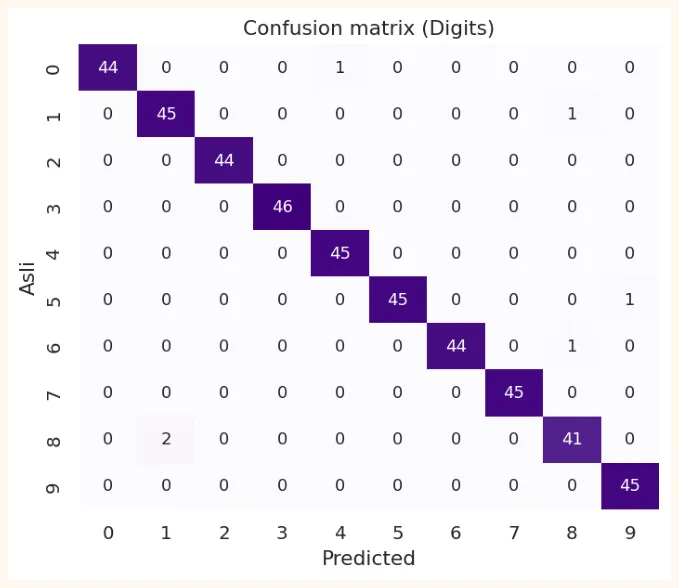
Confusion matrix batati hai ke model kin do classes me confuse hota hai:
import seaborn as sns
cm = confusion_matrix(y_te, pred)
fig, ax = plt.subplots(figsize=(6.2, 5))
sns.heatmap(cm, annot=True, fmt="d", cmap="Purples", cbar=False, ax=ax)
ax.set_xlabel("Predicted")
ax.set_ylabel("Asli")
ax.set_title("Confusion matrix (Digits)")
plt.show()
errors = np.where(pred != y_te)[0]
print("Ghalat predictions:", len(errors), "/", len(y_te))
OUTPUT
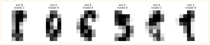
Ghalat predictions: 6 / 450
OUTPUT (chart)
Error analysis: ghalat prediction wali tasveerein khud dekho. Aksar wajah saaf nazar aati hai (kharab likhai, do number milte julte):
n = min(8, len(errors))
fig, axes = plt.subplots(1, n, figsize=(10, 1.9))
for ax, idx in zip(np.atleast_1d(axes), errors[:n]):
    ax.imshow(im_te[idx], cmap="gray_r", interpolation="nearest")
    ax.set_title("asli %d\nmodel %d" % (y_te[idx], pred[idx]), fontsize=9)
    ax.axis("off")
    plt.tight_layout()
    plt.show()
OUTPUT (chart)
Is ke baad model save karo. Keras me .keras format hai, aur aage hum ise predict function me lapet dete hain:
model.save("digits_cnn.keras")                    # Keras model
loaded = keras.models.load_model("digits_cnn.keras")
def predict_digit(img_8x8):
    x = (img_8x8 / 16.0).reshape(1, 8, 8, 1)       # wohi preprocessing jo training me thi
    probs = loaded.predict(x, verbose=0)[0]
    return int(probs.argmax()), float(probs.max())
24.8 Fashion-MNIST: ek poora Keras image project (Colab)
Fashion-MNIST : 70,000 kapdon ki 28x28 greyscale tasveerein, 10 qismein (60,000 train, 10,000 test). Ye data Keras khud download karta hai, is liye isay Colab me chalao .
from tensorflow import keras
from tensorflow.keras import layers
import numpy as np
(X_train, y_train), (X_test, y_test) = keras.datasets.fashion_mnist.load_data()
print(X_train.shape, y_train.shape, X_test.shape)
class_names = ["T-shirt/top", "Trouser", "Pullover", "Dress", "Coat",
"Sandal", "Shirt", "Sneaker", "Bag", "Ankle boot"]
X_train = X_train[..., np.newaxis] / 255.0     # (60000, 28, 28, 1), 0 se 1
X_test  = X_test[..., np.newaxis] / 255.0
print(X_train.shape, X_train.max())
OUTPUT (namoona)
(60000, 28, 28) (60000,) (10000, 28, 28)
(60000, 28, 28, 1) 1.0
model = keras.Sequential([
    keras.Input(shape=(28, 28, 1)),
    layers.Conv2D(32, 3, activation="relu"),
    layers.MaxPooling2D(),
    layers.Conv2D(64, 3, activation="relu"),
    layers.MaxPooling2D(),
    layers.Flatten(),
    layers.Dropout(0.3),
    layers.Dense(10, activation="softmax"),
])
model.compile(optimizer="adam",
              loss="sparse_categorical_crossentropy", metrics=["accuracy"])
model.summary()
OUTPUT (namoona)
Model: "sequential"
| Layer (type) | Output shape | Param # |
|---|---|---|
| conv2d (Conv2D) | (None, 26, 26, 32) | 320 |
| max_pooling2d (MaxPooling2D) | (None, 13, 13, 32) | 0 |
| conv2d_1 (Conv2D) | (None, 11, 11, 64) | 18,496 |
| max_pooling2d_1 (MaxPooling2D) | (None, 5, 5, 64) | 0 |
| flatten (Flatten) | (None, 1600) | 0 |
| dropout (Dropout) | (None, 1600) | 0 |
| dense (Dense) | (None, 10) | 16,010 |
| Total params | 34,826 (136.04 KB) | |
| Trainable params | 34,826 (136.04 KB) | |
| Non-trainable params | 0 (0.00 B) |
24.9 Apne folders se images load karna
Asli project me tasveerein folders me hoti hain, har class ka ek folder. Keras unhein seedha load kar leta hai:
dataset/
  train/
    cat/  img1.jpg  img2.jpg ...
    dog/  img1.jpg ...
  val/
    cat/ ...
    dog/ ...
train_ds = keras.utils.image_dataset_from_directory(
    "dataset/train", image_size=(160, 160), batch_size=32)
val_ds = keras.utils.image_dataset_from_directory(
    "dataset/val", image_size=(160, 160), batch_size=32)
print(train_ds.class_names)        # folder ke naam = classes
train_ds = train_ds.prefetch(buffer_size=tf.data.AUTOTUNE)   # tez loading (import
tensorflow as tf)
Colab me GPU lagao: Runtime > Change runtime type > GPU. CNN training CPU par bohat dheemi hoti hai.
24.10 Aam Galtiyan aur Hands-on
AAM GALTIYAN
-
Pre-trained model ki preprocessing bhoolna (har model ki apni
preprocess_inputhoti hai). -
Base ko freeze kiye baghair train karna , jis se seekhe hue weights pehle hi epoch me kharab ho jate hain.
-
Fine-tuning me bara learning rate.
-
Test accuracy par bharosa jab ke validation aur test ka data overlap karta ho.
-
Sirf accuracy dekhna; confusion matrix aur ghalat tasveerein bhi dekho.
-
Prediction me alag preprocessing (training me /255 aur prediction me nahi).
Hands-on
-
Parameters ginna:
Conv2D(64, 3x3)jo 32 channels par chale, aur depthwise separable version, dono ke parameters nikal kar muqabla karo. -
ResNet block: Functional API se 2 residual blocks wala chhota network banao aur
model.summary()dekho. -
Transfer Learning: Colab me 3 class (maslan chai, biryani, burger) ki 30-30 tasveerein folders me rakh kar MobileNetV2 se classifier banao.
-
Fashion-MNIST: upar wala CNN chalao, confusion matrix banao aur batao kaun si do classes sab se zyada confuse hoti hain.
-
Fine-tuning: feature extraction ke baad aakhri 30 layers unfreeze kar ke dekho accuracy badhti hai ya nahi.
KEY TAKEAWAYS
-
LeNet se EfficientNet tak har architecture ne ek masla hal kiya: gehrai (ResNet), kam computation (Inception, MobileNet).
-
Skip connection
F(x) + xgradient ko seedha peeche pohanchata hai, jis se 50-100+ layers ka network train hota hai. -
1x1 convolution aur depthwise separable convolution parameters aur computation bohat kam kar dete hain.
-
Global Average Pooling Flatten + bari Dense se kam parameters rakhta hai aur overfitting kam karta hai.
-
Transfer Learning: pre-trained base freeze karo, naya head train karo; phir zaroorat par chhote lr se finetune.
-
Image project ka dhancha: data, baseline, model, evaluation, confusion matrix, error analysis, save aur predict.
-
Training aur prediction ki preprocessing hamesha ek jaisi rakho.