Chapter 12: Introduction to Machine Learning
MODULE 4 | WEEK 12
Chapter 12: Introduction to Machine Learning
We have now arrived at the place this whole journey was leading to: Machine Learning (ML) . Everything you learned in the earlier modules about Python, Pandas, statistics and regression will be put to use here. In this chapter we will learn the basic idea of ML, its types, the way scikit-learn works , and the basic principles for evaluating a model.
12.1 What is Machine Learning?
In Machine Learning we do not give the computer rules written by hand . Instead we give it examples (data) , and it learns the patterns hidden in those examples by itself, which it then uses on new data .
Basic terms
| Term | Meaning | Example (house price) |
|---|---|---|
| Sample / Row | One example | One house |
| Features (X) | The input columns used to make the prediction | Size, rooms, age, city |
| Target / Label (y) | What we want to predict | House price |
| Training | The model learning from data | model.fit(X_train, y_train) |
| Parameters | What the modellearns by itself | Regression coefficients |
| Hyperparameters | Whatwe decide in advance | Tree depth, k in KNN, regularization alpha |
| Prediction | A guess on new data | model.predict(X_new) |
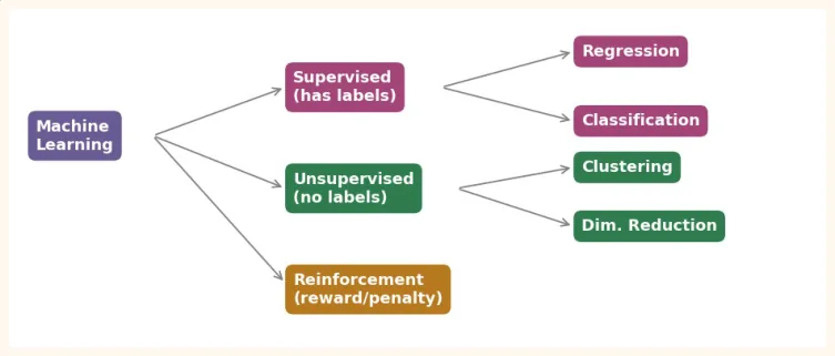
12.2 Types of ML
1) Supervised Learning (learning with supervision)
The data also contains the answer (label) . The model learns the relationship from input to answer . There are two kinds of problems:
| Problem | What the target is | Example | Algorithms |
|---|---|---|---|
| Regression | Anumber(continuous) | House price, tomorrow's temperature, sales | Linear Regression, Random Forest... |
| Classification | Acategory(class) | Spam or not spam, sick or not sick, Iris l | Logistic Regression, Decision Tree, |
| flower | SVM, KNN... |
2) Unsupervised Learning (learning without supervision)
The data has no label . The model finds the hidden structure in the data on its own.
-
Clustering: making groups of similar things (groups of customers). Chapter 16.
-
Dimensionality Reduction: reducing the number of columns while keeping the information (PCA). Chapter 17.
-
Anomaly detection: finding strange/unusual things (fraud).
3) Reinforcement Learning (learning from reward and penalty)
An agent takes an action in an environment, and gets a reward or penalty for its performance. Over time the agent learns the actions that earn more reward. Examples: an AI playing a game, a robot learning to walk. In this course we only get to know it.
import matplotlib.pyplot as plt
fig, ax = plt.subplots(figsize=(9, 3.6))
ax.axis("off")
boxes = [
    (0.0, 0.55, "Machine\nLearning", "#6B5B95"),
    (0.33, 0.78, "Supervised\n(has labels)", "#A4457A"),
    (0.33, 0.30, "Unsupervised\n(no labels)", "#2F7D4F"),
    (0.33, -0.18, "Reinforcement\n(reward/penalty)", "#B7791F"),
    (0.70, 0.95, "Regression", "#A4457A"),
    (0.70, 0.62, "Classification", "#A4457A"),
    (0.70, 0.40, "Clustering", "#2F7D4F"),
    (0.70, 0.12, "Dim. Reduction", "#2F7D4F"),
]
for x, y, t, c in boxes:
    ax.text(x, y, t, ha="left", va="center", fontsize=10, color="white", fontweight="bold",
            bbox=dict(boxstyle="round,pad=0.5", fc=c, ec="none"))
for src, dst in [((0.15, 0.55), (0.32, 0.78)), ((0.15, 0.55), (0.32, 0.30)), ((0.15, 0.55),
(0.32, -0.15)),
((0.52, 0.78), (0.69, 0.95)), ((0.52, 0.78), (0.69, 0.62)), ((0.54, 0.30), (0.69, 0.40)), ((0.54, 0.30), (0.69, 0.12))]: ax.annotate("", xy=dst, xytext=src, arrowprops=dict(arrowstyle="->", color="gray")) ax.set_xlim(-0.02, 1.0) ax.set_ylim(-0.4, 1.1) plt.show() OUTPUT (chart)
12.3 The complete ML Workflow
This is the same Data Science Pipeline you saw in Chapter 1, now from the ML point of view:
-
Define the problem: is it regression or classification? What will be the measure of success?
-
Collect and understand the data (EDA) .
-
Clean the data: missing values, duplicates, outliers.
-
Train/Test split (no "learning" step before this!).
-
Preprocessing / Feature engineering: scaling, encoding, new features.
-
Choose a model and train it.
-
Evaluate (on the test set) and improve (hyperparameter tuning).
-
Deploy and monitor.
12.4 The scikit-learn way
scikit-learn (sklearn) is Python's most popular ML library. Its best feature: every algorithm has the same interface . Once you learn it, you can use any algorithm.
| Method | Job | When |
|---|---|---|
| model.fit(X, y) | Learn from data (training) | On every model |
| model.predict(X) | Make predictions | On supervised models |
| model.score(X, y) | Default metric (accuracy for classification, R² for regression) | On supervised models |
| transformer.fit(X) | Learn something from data (like mean, std) | Scaler, Encoder, PCA |
| transformer.transform(X) | Change data using what was learned | Scaler, Encoder, PCA |
| transformer.fit_transform(X) | Both together (on train data only) | Scaler, Encoder, PCA |
First, a classic dataset: Iris . 4 measurements of 150 flowers (petal/sepal length and width) and 3 species (setosa, versicolor, virginica). Question: tell the species from the measurements (classification).
import numpy as np
import pandas as pd
from sklearn.datasets import load_iris
iris = load_iris(as_frame=True)
X = iris.data # features (DataFrame) y = iris.target # target (0, 1, 2) print(X.shape, y.shape) print(X.head(3)) print(iris.target_names) print(y.value_counts()) OUTPUT (150, 4) (150,) sepal length (cm) sepal width (cm) petal length (cm) \ 0 5.1 3.5 1.4 1 4.9 3.0 1.4 2 4.7 3.2 1.3 petal width (cm) 0 0.2 1 0.2 2 0.2 ['setosa' 'versicolor' 'virginica'] target 0 50 1 50 2 50 Name: count, dtype: int64
Your first ML model: in 5 lines
from sklearn.model_selection import train_test_split
from sklearn.neighbors import KNeighborsClassifier
X_train, X_test, y_train, y_test = train_test_split(
    X, y, test_size=0.2, random_state=42, stratify=y)
model = KNeighborsClassifier() # 1) create the model model.fit(X_train, y_train) # 2) learn pred = model.predict(X_test) # 3) make predictions print("First 5 predictions:", pred[:5]) print("Actual answers :", y_test.values[:5]) print("Accuracy:", round(model.score(X_test, y_test), 3)) # 4) evaluate OUTPUT First 5 predictions: [0 2 1 1 0] Actual answers : [0 2 1 1 0] Accuracy: 1.0
Change the model: the interface stays the same
from sklearn.linear_model import LogisticRegression
from sklearn.tree import DecisionTreeClassifier
from sklearn.ensemble import RandomForestClassifier
models = {
    "Logistic Regression": LogisticRegression(max_iter=1000),
    "Decision Tree": DecisionTreeClassifier(random_state=0),
    "Random Forest": RandomForestClassifier(random_state=0),
    "KNN": KNeighborsClassifier(),
}
for name, m in models.items():
m.fit(X_train, y_train) print(f"{name:20s} accuracy: {m.score(X_test, y_test):.3f}") OUTPUT Logistic Regression accuracy: 0.967 Decision Tree accuracy: 0.967 Random Forest accuracy: 0.933 KNN accuracy: 1.000
See how only the model name changed and the rest of the code stayed the same. This is why scikit-learn is so popular.
12.5 Train/Test Split and Data Leakage
In the previous module you saw that testing a model on the same data it learned from is a fraud. The test set is the "exam" the model has never seen before. A very big mistake is Data Leakage : information from the test data quietly getting into training .
The most common leakage: scaling the whole data
from sklearn.preprocessing import StandardScaler
# WRONG (leakage): the mean/std of the whole data also comes from the test set # scaler = StandardScaler().fit(X) # <- includes test information # RIGHT: learn only from train, only apply on test scaler = StandardScaler() X_train_s = scaler.fit_transform(X_train) # fit + transform (train) X_test_s = scaler.transform(X_test) # transform only (test) print("Train mean (approx. 0):", X_train_s.mean(axis=0).round(2)) print("Test mean (not 0): ", X_test_s.mean(axis=0).round(2)) OUTPUT Train mean (approx. 0): [-0. -0. 0. 0.] Test mean (not 0): [ 0.01 0.1 -0.03 -0.04]
12.6 Preprocessing: getting data ready for the model
ML models understand only numbers , and many models are affected by the scale of numbers. That is why the data has to be prepared.
1) Feature Scaling
If one feature is between 0 and 1 (like a percentage) and another between 0 and 1,000,000 (like a salary), then models that work on distance (KNN, SVM, Gradient Descent, PCA) give more importance to the big values.
| Scaler | What it does | When |
|---|---|---|
| StandardScaler | Mean 0, std 1 (z-score) | Usually the first choice, Normal-like data |
| MinMaxScaler | Between 0 and 1 | When limits are known, neural networks |
| RobustScaler | Uses median and IQR | When there are outliers |
Trees and Random Forest do not need scaling. Linear models, KNN, SVM, PCA and neural networks do.
2) Turning categorical data into numbers (Encoding)
cars = pd.DataFrame({
    "fuel": ["Petrol", "Diesel", "Petrol", "CNG"],
    "size": ["Small", "Large", "Medium", "Small"],
})
# One-Hot: a separate 0/1 column for each category (for nominal data)
print(pd.get_dummies(cars["fuel"]).astype(int))
# Ordinal: for categories with an order (Small < Medium < Large) cars["size_num"] = cars["size"].map({"Small": 1, "Medium": 2, "Large": 3}) print(cars) OUTPUT CNG Diesel Petrol 0 0 0 1 1 0 1 0 2 0 0 1 3 1 0 0 fuel size size_num 0 Petrol Small 1 1 Diesel Large 3 2 Petrol Medium 2 3 CNG Small 1
from sklearn.preprocessing import OneHotEncoder
enc = OneHotEncoder(sparse_output=False, handle_unknown="ignore") print(enc.fit_transform(cars[["fuel"]])) print(enc.get_feature_names_out()) OUTPUT [[0. 0. 1.] [0. 1. 0.] [0. 0. 1.] [1. 0. 0.]] ['fuel_CNG' 'fuel_Diesel' 'fuel_Petrol']
3) Missing values
from sklearn.impute import SimpleImputer
data = np.array([[1.0, 10], [2.0, np.nan], [np.nan, 30], [4.0, 40]])
imp = SimpleImputer(strategy="median")      # "mean", "median", "most_frequent", "constant"
print(imp.fit_transform(data))
OUTPUT [[ 1. 10.] [ 2. 30.] [ 2. 30.] [ 4. 40.]]
All in one: Pipeline and ColumnTransformer (a glimpse)
You can pack different preprocessing for different columns, and then running the model, into a single object. The benefit: no leakage and clean code. We will work on this fully in Chapters 19 and 20; for now just a glimpse:
from sklearn.pipeline import Pipeline from sklearn.compose import ColumnTransformer from sklearn.linear_model import LogisticRegression df = pd.DataFrame({ "age": [25, 32, np.nan, 41, 29, 52, 36, 47], "city": ["K", "L", "K", "I", "L", "K", "I", "L"], "bought": [0, 1, 0, 1, 0, 1, 1, 0], }) X_df, y_s = df[["age", "city"]], df["bought"] prep = ColumnTransformer([ ("num", Pipeline([("imp", SimpleImputer(strategy="median")), ("sc", StandardScaler())]), ["age"]), ("cat", OneHotEncoder(handle_unknown="ignore"), ["city"]), ]) pipe = Pipeline([("prep", prep), ("model", LogisticRegression())]) pipe.fit(X_df, y_s) # everything in one go print(pipe.predict(X_df)[:4]) OUTPUT [0 0 0 1]
12.7 Overfitting and Underfitting
This is the most basic problem of ML, and every algorithm gets caught in it.
12.8 Basic principles of Model Evaluation
1) Baseline (the simplest model)
Before building any model, ask: what is the simplest guess without any ML? In classification, "always say the most common class"; in regression, "always say the average". Only by comparing with this can your model be judged good or bad.
from sklearn.dummy import DummyClassifier
base = DummyClassifier(strategy="most_frequent").fit(X_train, y_train)
print("Baseline accuracy :", round(base.score(X_test, y_test), 3))      # ~ 1/3 (three equal
classes)
rf = RandomForestClassifier(random_state=0).fit(X_train, y_train)
print("Random Forest :", round(rf.score(X_test, y_test), 3)) OUTPUT Baseline accuracy : 0.333 Random Forest : 0.933
2) Accuracy and its limit
Accuracy = correct predictions / total predictions . But when the classes are not balanced (imbalanced), accuracy can deceive . If 99% of people are healthy and 1% are sick, a model that always says "healthy" has 99% accuracy, but it is useless because it does not catch even one sick person. That is why Chapter 14 brings precision, recall, F1, ROC-AUC .
3) Cross-Validation (do not trust a single split)
With just one train/test split the result can depend on luck (maybe easy examples ended up in the test set). KFold Cross-Validation divides the data into K parts (folds); each time one part is the test and the rest is train. At the end you get the average and the spread of K scores, which is more trustworthy.
12.9 Hands-on
A complete small workflow on the Breast cancer dataset (569 patients, 30 measurements, target: malignant or benign):
from sklearn.datasets import load_breast_cancer
bc = load_breast_cancer(as_frame=True) Xb, yb = bc.data, bc.target print(Xb.shape, "| malignant:", int((yb == 0).sum()), "| benign:", int((yb == 1).sum())) OUTPUT
(569, 30) | malignant: 212 | benign: 357
-
Split: 80/20, stratify=yb , random_state=42.
-
Baseline: find the accuracy of DummyClassifier.
-
Scaling: apply StandardScaler (fit on train only).
-
Models: run both KNN and LogisticRegression on scaled and unscaled data. See the difference scaling makes.
-
Cross-validation: find the 5-fold CV score of the best model.
-
Thinking question: why is accuracy not enough in cancer detection? (Hint: what is the cost of missing a sick patient?)
Xtr, Xte, ytr, yte = train_test_split(Xb, yb, test_size=0.2, random_state=42, stratify=yb)
print("Baseline:", round(DummyClassifier(strategy="most_frequent").fit(Xtr, ytr).score(Xte,
yte), 3))
for name, model in [("KNN", KNeighborsClassifier()), ("LogReg",
LogisticRegression(max_iter=5000))]:
    raw = model.fit(Xtr, ytr).score(Xte, yte)
    sc = StandardScaler().fit(Xtr)
    scaled = model.fit(sc.transform(Xtr), ytr).score(sc.transform(Xte), yte)
    print(f"{name:7s} unscaled = {raw:.3f} | scaled = {scaled:.3f}")
OUTPUT
Baseline: 0.632
KNN     unscaled = 0.912 | scaled = 0.956
LogReg  unscaled = 0.965 | scaled = 0.982
KEY TAKEAWAYS
-
In ML we learn patterns from examples so that we can predict correctly on new data (generalization).
-
• Supervised (has labels: regression or classification), Unsupervised (no labels: clustering, dimensionality reduction), Reinforcement (reward/penalty).
-
Predict the target (y) from the features (X). The model learns parameters, we decide hyperparameters.
-
scikit-learn: fit, predict, score, transform. Every model has the same interface.
-
Always do a train/test split. fit only on train, transform on both (avoid leakage).
-
Scaling (StandardScaler), encoding (OneHot), imputation (SimpleImputer). Trees do not need scaling.
-
Underfitting = too simple, overfitting = memorizing. The test score is the real score. Always use a baseline and cross-validation.