Chapter 18: Support Vector Machines (SVM)
MODULE 4 | WEEK 18
Chapter 18: Support Vector Machines (SVM)
Support Vector Machine (SVM) is a powerful and elegant classification algorithm. Its way is different from logistic regression and trees: it finds the widest road (margin) between two classes. And thanks to the kernel trick , it can also make curvy, complex boundaries.
18.1 The SVM idea: the widest road
Between two classes many lines can be drawn that separate them. The question is: which one is the best? SVM says: the line that is farthest from both classes , that is, the one that has the widest empty road (margin) on both sides.
18.2 Hard margin and Soft margin: C
In real data the classes are often mixed and cannot be separated perfectly. If we insist that not a single point should be inside the margin or on the wrong side ( hard margin ), then either the problem cannot be solved at all or the boundary becomes very narrow and dependent on noise.
In a soft margin we tolerate some mistakes , and the parameter C tells how many:
| C | Meaning | Margin | Risk |
|---|---|---|---|
| Small C(like 0.01) | Tolerates mistakes, prefers the margin | Wide, simple | Underfitting |
| Large C(like 1000) | Harsh penalty for mistakes, wants every point right | Narrow | Overfitting |
18.3 The Kernel Trick: curvy boundaries
Sometimes it is not possible at all to separate the data with a straight line . Look at the classes below, one inside the other (concentric circles):
from sklearn.datasets import make_circles
Xc, yc = make_circles(n_samples=200, factor=0.3, noise=0.08, random_state=0)
lin = SVC(kernel="linear").fit(Xc, yc)
plt.figure(figsize=(5.4, 4.6))
plt.scatter(Xc[:, 0], Xc[:, 1], c=yc, cmap="coolwarm", edgecolor="white")
plt.title(f"A straight line does not work here (accuracy {lin.score(Xc, yc):.2f})")
plt.show()
OUTPUT (chart)
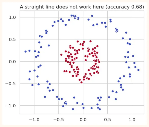
A straight line cannot separate this. The wonder of the kernel trick : take the data to more dimensions where it can be separated by a straight line (or plane), and when you come back the boundary looks curvy.
OUTPUT (chart)
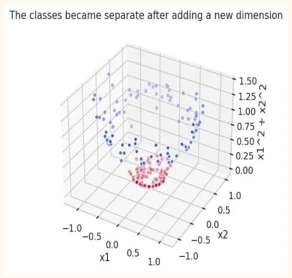
After adding the new (third) dimension x1² + x2² , the red points came down and the blue ones up , and a straight plane can separate them. The kernel does all this without actually creating new columns .
Common kernels
| Kernel | Shape of the boundary | When |
|---|---|---|
| linear | Straight line / plane | The data is almost linearly separable, very many features |
| poly(degree = d) | Polynomial curve | When the relationship is polynomial (rarely used) |
| rbf(default) | Curvy, any shape | Usually the first choice, when you do not know what the data is like |
| sigmoid | Like a neural network | Rarely used |
from sklearn.inspection import DecisionBoundaryDisplay
from sklearn.datasets import make_moons
Xm, ym = make_moons(n_samples=200, noise=0.2, random_state=1)
fig, axes = plt.subplots(1, 3, figsize=(13, 4))
for ax, (kernel, kw) in zip(axes, [("linear", {}), ("poly", {"degree": 3}), ("rbf", {})]):
    m = SVC(kernel=kernel, C=1, **kw).fit(Xm, ym)
    DecisionBoundaryDisplay.from_estimator(m, Xm, ax=ax, alpha=0.35, cmap="coolwarm",
response_method="predict")
    ax.scatter(Xm[:, 0], Xm[:, 1], c=ym, cmap="coolwarm", edgecolor="white", s=22)
    ax.set_title(f"{kernel}  (accuracy {m.score(Xm, ym):.2f})")
plt.tight_layout()
plt.show()
OUTPUT (chart)
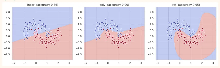
gamma of the RBF kernel
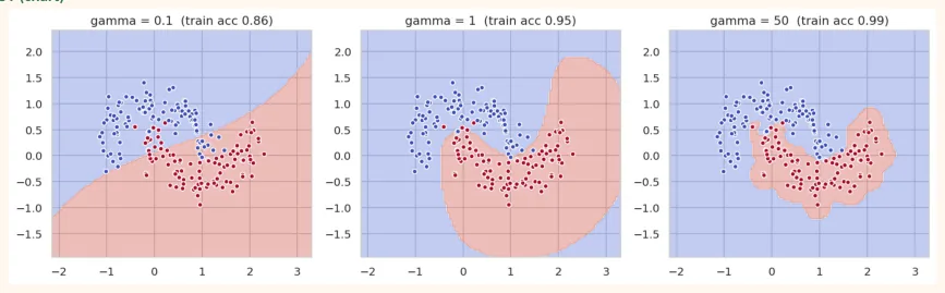
The RBF kernel has one more important hyperparameter, gamma : it tells how far the influence of one point reaches.
-
Small gamma: the influence of every point reaches far (the boundary is delicate, simple, smooth) → danger of underfitting.
-
Large gamma: the influence of every point is only nearby (the boundary wraps around every point, very complex) → danger of overfitting.
fig, axes = plt.subplots(1, 3, figsize=(13, 4))
for ax, g in zip(axes, [0.1, 1, 50]):
    m = SVC(kernel="rbf", gamma=g, C=1).fit(Xm, ym)
    DecisionBoundaryDisplay.from_estimator(m, Xm, ax=ax, alpha=0.35, cmap="coolwarm",
response_method="predict")
    ax.scatter(Xm[:, 0], Xm[:, 1], c=ym, cmap="coolwarm", edgecolor="white", s=22)
    ax.set_title(f"gamma = {g}  (train acc {m.score(Xm, ym):.2f})")
plt.tight_layout()
plt.show()
OUTPUT (chart)
18.4 SVC in scikit-learn
On the breast cancer dataset. Remember: scaling is necessary in SVM , because it works on distance.
from sklearn.datasets import load_breast_cancer
from sklearn.model_selection import train_test_split
from sklearn.preprocessing import StandardScaler
from sklearn.pipeline import make_pipeline
bc = load_breast_cancer(as_frame=True)
X_train, X_test, y_train, y_test = train_test_split(bc.data, bc.target, test_size=0.25,
random_state=0, stratify=bc.target)
no_scale = SVC().fit(X_train, y_train)
scaled = make_pipeline(StandardScaler(), SVC()).fit(X_train, y_train)
print("Without scaling:", round(no_scale.score(X_test, y_test), 3)) print("With scaling :", round(scaled.score(X_test, y_test), 3)) OUTPUT Without scaling: 0.916 With scaling : 0.958 Scaling improved the result a lot. Now the different kernels:
for kernel in ["linear", "poly", "rbf", "sigmoid"]: m = make_pipeline(StandardScaler(), SVC(kernel=kernel)).fit(X_train, y_train) print(f"{kernel:8s} test accuracy = {m.score(X_test, y_test):.3f}") OUTPUT linear test accuracy = 0.965 poly test accuracy = 0.909 rbf test accuracy = 0.958 sigmoid test accuracy = 0.930
Probability and multiclass
-
SVM usually gives only the class. With probability=True it also gives the probability (but training becomes slower).
-
SVM is really meant for two classes . For more classes scikit-learn itself applies the one-vs-one method (a separate SVM for every two classes).
from sklearn.datasets import load_iris
iris = load_iris() Xi_tr, Xi_te, yi_tr, yi_te = train_test_split(iris.data, iris.target, test_size=0.25, random_state=0, stratify=iris.target) m = make_pipeline(StandardScaler(), SVC(probability=True, random_state=0)).fit(Xi_tr, yi_tr) print("Iris accuracy:", round(m.score(Xi_te, yi_te), 3)) print("Probabilities of one flower:", m.predict_proba(Xi_te[:1]).round(3)) OUTPUT
Iris accuracy: 0.974
Probabilities of one flower: [[0.97  0.017 0.013]]
18.5 SVR: SVM for regression
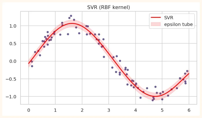
SVM can also predict numbers ( SVR ). The idea: make a tube (epsilon) and forgive the errors inside the tube, and penalize only the points outside the tube.
from sklearn.svm import SVR
rng = np.random.RandomState(0)
xr = np.sort(rng.uniform(0, 6, 80)).reshape(-1, 1)
yr = np.sin(xr).ravel() + rng.normal(0, 0.15, 80)
xs = np.linspace(0, 6, 300).reshape(-1, 1)
svr = SVR(kernel="rbf", C=10, epsilon=0.1).fit(xr, yr)
plt.figure(figsize=(7.5, 4))
plt.scatter(xr, yr, color="#6B5B95", s=16)
plt.plot(xs, svr.predict(xs), color="red", linewidth=2, label="SVR")
plt.fill_between(xs.ravel(), svr.predict(xs) - 0.1, svr.predict(xs) + 0.1, color="red",
alpha=0.15, label="epsilon tube")
plt.legend()
plt.title("SVR (RBF kernel)")
plt.show()
OUTPUT (chart)
18.6 A glimpse of Hyperparameter Tuning: GridSearchCV
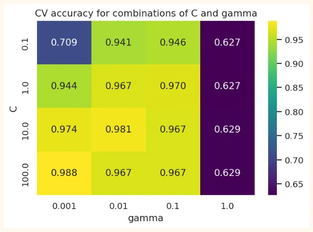
In SVM it is necessary to find the right combination of C and gamma . GridSearchCV tries different combinations with cross-validation and picks the best. (Its full details are in the next chapter.)
from sklearn.model_selection import GridSearchCV
pipe = make_pipeline(StandardScaler(), SVC()) grid = {"svc__C": [0.1, 1, 10, 100], "svc__gamma": [0.001, 0.01, 0.1, 1]} search = GridSearchCV(pipe, grid, cv=5, n_jobs=-1).fit(X_train, y_train) print("Best parameters:", search.best_params_) print("CV score:", round(search.best_score_, 3)) print("Test score:", round(search.score(X_test, y_test), 3)) OUTPUT Best parameters: {'svc__C': 100, 'svc__gamma': 0.001} CV score: 0.988 Test score: 0.958 scores = pd.DataFrame(search.cv_results_) heat = scores.pivot_table(index="param_svc__C", columns="param_svc__gamma", values="mean_test_score") import seaborn as sns plt.figure(figsize=(6.2, 4)) sns.heatmap(heat, annot=True, fmt=".3f", cmap="viridis") plt.title("CV accuracy for combinations of C and gamma") plt.ylabel("C") plt.xlabel("gamma") plt.show()
OUTPUT (chart)
18.7 Pros and cons of SVM
| Pros | Cons |
|---|---|
| Works well on data with many features | Very slow onbig data(hundreds of thousands of rows) |
| Curvy boundaries through kernels | Scaling isnecessary |
| Less overfitting because of the margin | Choosing C, gamma and kernel is hard |
| Memory efficient (only support vectors) | Does not give probability directly (extra computation) |
| Often the best on small and medium data | Hard to understand (kernel SVM is like a black box) |
| Popular where there are few samples and many features (like gene data) | Weak on noisy data and overlapping classes |
| When to choose SVM | When not to |
| Small or medium data, classes that separate cleanly | Hundreds of thousands of rows (Random Forest or Gradient Boosting is better) |
| Text classification (linear SVM) | When the model has to be explained (Logistic Regression or a Tree) |
| Many features and few samples | When probabilities are needed |
18.8 Hands-on
from sklearn.datasets import load_wine
wine = load_wine(as_frame=True) Xw_tr, Xw_te, yw_tr, yw_te = train_test_split(wine.data, wine.target, test_size=0.25, random_state=0, stratify=wine.target) print(wine.data.shape, "| classes:", np.bincount(wine.target)) for name, m in [("SVM without scaling", SVC()), ("SVM scaled", make_pipeline(StandardScaler(), SVC()))]: print(f"{name:22s} test accuracy = {m.fit(Xw_tr, yw_tr).score(Xw_te, yw_te):.3f}") OUTPUT (178, 13) | classes: [59 71 48] SVM without scaling test accuracy = 0.600 SVM scaled test accuracy = 1.000
-
Wine dataset (3 classes): see above how much scaling changed the accuracy. Write the reason in your own words (look at the scale of the features: wine.data.describe()).
-
Kernels: compare linear, poly and rbf on wine (scaled).
-
Effect of C: on breast cancer plot the train and test accuracy at C = 0.001, 0.01, 0.1, 1, 10, 100.
-
GridSearch: run a grid of C and gamma on wine and make a heatmap.
-
Comparison: find the 5-fold CV score of SVM, Logistic Regression and Random Forest on wine and make a table.
-
Thinking question: in the moons chart the train accuracy was very high at gamma = 50 . Will this model also do well on new data? How would you check?
from sklearn.model_selection import cross_val_score
from sklearn.linear_model import LogisticRegression
from sklearn.ensemble import RandomForestClassifier
for name, m in [("SVM", make_pipeline(StandardScaler(), SVC())), ("Logistic Regression", make_pipeline(StandardScaler(), LogisticRegression(max_iter=2000))), ("Random Forest", RandomForestClassifier(random_state=0))]: s = cross_val_score(m, wine.data, wine.target, cv=5) print(f"{name:20s} CV accuracy = {s.mean():.3f} (+/- {s.std():.3f})") OUTPUT
SVM                  CV accuracy = 0.983 (+/- 0.022)
Logistic Regression  CV accuracy = 0.983 (+/- 0.014)
Random Forest        CV accuracy = 0.983 (+/- 0.022)
KEY TAKEAWAYS
-
SVM finds the widest margin between two classes. Only the support vectors (points at the edge of the margin) decide the boundary.
-
C: the strictness of the soft margin. Small C = wide margin, simple (underfit). Large C = narrow margin, memorizing (overfit).
-
The kernel trick takes data to more dimensions to make curvy boundaries. rbf is usually the first choice; there are linear and poly too.
-
gamma in RBF: how far the influence of a point reaches. Small = smooth, large = around every point (overfit). Tune C and gamma together.
-
Scaling is necessary for SVM. For more classes one-vs-one is applied automatically; for probability use probability=True.
-
SVR is for regression (epsilon tube). Kernel SVM is slow on big data; best on small/medium data with many features.
-
GridSearchCV finds the best combination of C and gamma using cross-validation.