Chapter 16: Clustering (K-Means, Hierarchical, DBSCAN)
MODULE 4 | WEEK 16
Chapter 16: Clustering (K-Means, Hierarchical, DBSCAN)
Until now, in every problem we had the answer (label) . But often data has no label: a shop has 10,000 customers and nobody has said which one is of which type. Clustering (Unsupervised Learning) finds groups of similar things in the data by itself.
16.1 What is clustering?
Where is clustering used?
-
Customer segmentation: dividing customers into groups so that each group gets its own offers and marketing.
-
Grouping documents / news: similar topics in one place.
-
Image compression: reducing the colours of a picture.
-
Anomaly detection: whatever does not fit in any group is suspicious (fraud).
-
Biology: groups of similar genes or patients.
MUST REMEMBER
In clustering there is no correct answer to compare against. That is why it is unsupervised , and a human has to work out the meaning of the result ("this group is probably of people who look for cheap things").
16.2 K-Means Clustering
The most famous and simplest clustering algorithm. You have to say beforehand how many clusters (K) you want.
The steps of K-Means
-
Decide K (say 3) and pick K random points (centroids) from the data.
-
Put every data point into the cluster of its nearest centroid .
-
Find the new centroid of every cluster (the average of all the points in the cluster).
-
Repeat steps 2 and 3 until the centroids stop moving.
K-Means in scikit-learn
km = KMeans(n_clusters=3, n_init=10, random_state=42).fit(X) print("First 10 labels:", km.labels_[:10]) print("Centroids:") print(km.cluster_centers_.round(2)) print("Points in each cluster:", np.bincount(km.labels_)) print("Inertia:", round(km.inertia_, 1)) OUTPUT First 10 labels: [1 2 2 1 0 2 1 0 2 1] Centroids: [[ 9.63 0.54] [-8.55 5.57] [-1.26 4.38]] Points in each cluster: [100 100 100] Inertia: 573.4
Telling the cluster of new points
new_points = np.array([[0, 0], [-6, -8], [5, 5]]) print(km.predict(new_points)) OUTPUT [2 2 2]
How to choose K? The Elbow Method
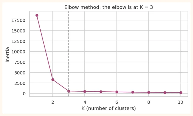
Inertia = the sum of the squares of each point's distance from its centroid (the lower, the tighter the clusters). Increasing K always lowers inertia (at K = number of points it is 0). We look for the K where the fall of inertia suddenly slows down : the bend of the elbow in the graph.
inertias = []
for k in range(1, 11):
    inertias.append(KMeans(n_clusters=k, n_init=10, random_state=0).fit(X).inertia_)
print([round(i) for i in inertias])
OUTPUT
[18700, 3303, 573, 501, 435, 374, 315, 273, 235, 210] plt.figure(figsize=(7, 3.8)) plt.plot(range(1, 11), inertias, marker="o", color="#A4457A") plt.axvline(3, color="gray", linestyle="--") plt.title("Elbow method: the elbow is at K = 3") plt.xlabel("K (number of clusters)") plt.ylabel("Inertia") plt.show() OUTPUT (chart)
Silhouette Score: how good is the clustering?
For every point: how close it is inside its own cluster (a) and how far it is from the nearest other cluster (b). Silhouette = (b - a) / max(a, b) .
-
Near +1: the point sits well inside its cluster, far from the others.
-
Near 0: on the border of two clusters.
-
Negative: probably in the wrong cluster.
from sklearn.metrics import silhouette_score
for k in range(2, 8):
    labels = KMeans(n_clusters=k, n_init=10, random_state=0).fit_predict(X)
    print(f"K = {k}: silhouette = {silhouette_score(X, labels):.3f}")
OUTPUT
K = 2: silhouette = 0.745
K = 3: silhouette = 0.790
K = 4: silhouette = 0.647
K = 5: silhouette = 0.471
K = 6: silhouette = 0.329
K = 7: silhouette = 0.349
The K with the highest silhouette is the best (here K = 3, which matches our true data). K is chosen by looking at both elbow and silhouette.
Requirements and weaknesses of K-Means
-
Scaling the features is necessary (because it works on distance).
-
It assumes clusters are round and of roughly equal size . It fails on long or curvy clusters.
-
K has to be given beforehand.
-
Outliers pull the centroid.
-
It depends on the start (that is why n_init).
from sklearn.preprocessing import StandardScaler
np.random.seed(0)
# age (20-60) and income (20,000-200,000): very different scales
age = np.random.uniform(20, 60, 200)
income = np.random.uniform(20000, 200000, 200)
people = pd.DataFrame({"age": age, "income": income})
raw_labels = KMeans(n_clusters=3, n_init=10, random_state=0).fit_predict(people)
scaled = StandardScaler().fit_transform(people)
sc_labels = KMeans(n_clusters=3, n_init=10, random_state=0).fit_predict(scaled)
# Unscaled, age has no effect: clusters are formed by income alone
print("Unscaled: average age in each cluster:",
      people.groupby(raw_labels)["age"].mean().round(1).to_dict())
print("Scaled  : average age in each cluster:",
      people.groupby(sc_labels)["age"].mean().round(1).to_dict())
OUTPUT
Unscaled: average age in each cluster: {0: 41.0, 1: 39.2, 2: 39.8}
Scaled  : average age in each cluster: {0: 46.8, 1: 46.8, 2: 27.1}
In the unscaled data the income numbers are in the thousands and age is from 20 to 60, so only income shows up in the distance, and the clusters do not show much difference in age. After scaling both features get equal importance.
16.3 Hierarchical Clustering
In K-Means we had to give K first. Hierarchical Clustering builds a family tree in which all the points join one by one, and then we decide where to cut the tree.
The Agglomerative (bottom-up) way
-
At the start every point is its own cluster .
-
Join the two nearest clusters .
-
Repeat until everything becomes one cluster .
Ways of measuring the distance between two clusters ( linkage ):
| Linkage | How the distance is measured | Characteristics |
|---|---|---|
| ward(the usual default) | The join that increases the spread inside the cluster the least | Round clusters of equal size, usually the best |
| single | The nearest points of the two clusters | Clusters in long chains, but affected by noise |
| complete | The farthest points | Small, round clusters |
| average | The average of all pairs | In between |
Dendrogram
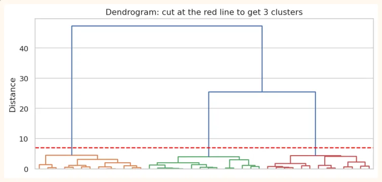
The picture of the tree is called a dendrogram . At the bottom is every point, and above are the joining clusters. The height of a vertical line shows how far apart two clusters were when they joined. If you cut with a horizontal line , the clusters left at that moment are our clusters.
from scipy.cluster.hierarchy import dendrogram, linkage, fcluster
Xs, _ = make_blobs(n_samples=40, centers=3, cluster_std=0.9, random_state=3) Z = linkage(Xs, method="ward") plt.figure(figsize=(9, 4)) dendrogram(Z, color_threshold=7, no_labels=True) plt.axhline(7, color="red", linestyle="--") plt.title("Dendrogram: cut at the red line to get 3 clusters") plt.ylabel("Distance") plt.show() OUTPUT (chart)
from sklearn.cluster import AgglomerativeClustering
agg = AgglomerativeClustering(n_clusters=3, linkage="ward").fit(Xs) print("Cluster sizes:", np.bincount(agg.labels_)) print("Also from scipy fcluster:", np.bincount(fcluster(Z, t=3, criterion="maxclust"))[1:]) OUTPUT Cluster sizes: [13 13 14] Also from scipy fcluster: [13 14 13]
Pro: no need to give K beforehand, and the dendrogram shows the whole structure of the data. Con: slow on big data (more than thousands of rows), and points once joined are never separated again.
16.4 DBSCAN: density-based clustering
K-Means and hierarchical like round clusters. But in real data clusters can be of any shape , and there is also noise . DBSCAN (Density-Based Spatial Clustering of Applications with Noise) makes clusters out of densely populated areas .
An easy way to choose eps: the k-distance plot
from sklearn.neighbors import NearestNeighbors
nn = NearestNeighbors(n_neighbors=6).fit(Xm) dist, _ = nn.kneighbors(Xm) kdist = np.sort(dist[:, -1]) print("Distance to the 6th neighbour: median =", kdist[len(kdist)//2].round(3), "| 95th percentile =", np.percentile(kdist, 95).round(3)) OUTPUT
Distance to the 6th neighbour: median = 0.08 | 95th percentile = 0.174 The usual way: find each point's distance to its min_samples-th neighbour , sort them, and where the graph shows a sudden jump , that is a good estimate for eps. The numbers above show that for most points the distance is small, and for a few (noise) it is very large.
16.5 Comparing the three algorithms
| K-Means | Hierarchical | DBSCAN | |
|---|---|---|---|
| Must K be given? | Yes | Decided at the end by cutting | No (needs eps and min_samples) |
| Shape of clusters | Round | Mostly round (depends on linkage) | Any shape |
| Noise / outliers | Cannot handle | Cannot handle | Recognises by itself |
| On big data | Fast | Slow | Medium |
| Output | Labels directly | The whole tree (dendrogram) | Labels and -1 (noise) |
| When to use | Big data, round groups | Small data, when you want to see the structure | Strange shapes, data with noise |
16.6 Mini Project: Customer Segmentation
Synthetic (made-up) data of 300 customers of a mall: age, annual income, and spending score (1 to 100, how much they spend). Goal: find groups of customers so that each group gets its own marketing.
rng = np.random.RandomState(10) groups = [ (rng.normal(25, 3, 70), rng.normal(35, 6, 70), rng.normal(75, 8, 70)), # young, low income, high spending (rng.normal(45, 5, 80), rng.normal(95, 10, 80), rng.normal(80, 7, 80)), # rich, high spending (rng.normal(50, 6, 80), rng.normal(90, 10, 80), rng.normal(22, 8, 80)), # rich, low spending (rng.normal(30, 5, 70), rng.normal(30, 6, 70), rng.normal(25, 8, 70)), # low income, low spending ] customers = pd.DataFrame({ "age": np.concatenate([g[0] for g in groups]), "income_k": np.concatenate([g[1] for g in groups]), "spending": np.concatenate([g[2] for g in groups]), }).clip(lower=1).round(1) print(customers.shape) print(customers.describe().round(1)) OUTPUT (300, 3) age income_k spending count 300.0 300.0 300.0 mean 38.1 64.8 50.1 std 11.0 32.0 28.1 min 19.1 13.1 6.1 25% 27.4 32.4 23.1 50% 40.0 78.2 44.8 75% 47.2 95.2 78.6 max 63.5 121.8 96.7
Step 1: Scale and choose K
from sklearn.preprocessing import StandardScaler
Xc = StandardScaler().fit_transform(customers)
for k in range(2, 8):
    lab = KMeans(n_clusters=k, n_init=10, random_state=0).fit_predict(Xc)
    print(f"K = {k}: inertia = {KMeans(n_clusters=k, n_init=10,
random_state=0).fit(Xc).inertia_:7.1f} | silhouette = {silhouette_score(Xc, lab):.3f}")
OUTPUT
K = 2: inertia =   386.5 | silhouette = 0.531
K = 3: inertia =   212.9 | silhouette = 0.586
K = 4: inertia =    89.6 | silhouette = 0.659
K = 5: inertia =    77.0 | silhouette = 0.580
K = 6: inertia =    67.0 | silhouette = 0.520
K = 7: inertia =    57.5 | silhouette = 0.434
Step 2: The model, and understanding each group
final = KMeans(n_clusters=4, n_init=10, random_state=0).fit(Xc)
customers["segment"] = final.labels_
profile = customers.groupby("segment").agg( customers=("age", "count"), avg_age=("age", "mean"), avg_income_k=("income_k", "mean"), avg_spending=("spending", "mean"), ).round(1) print(profile) OUTPUT customers avg_age avg_income_k avg_spending segment
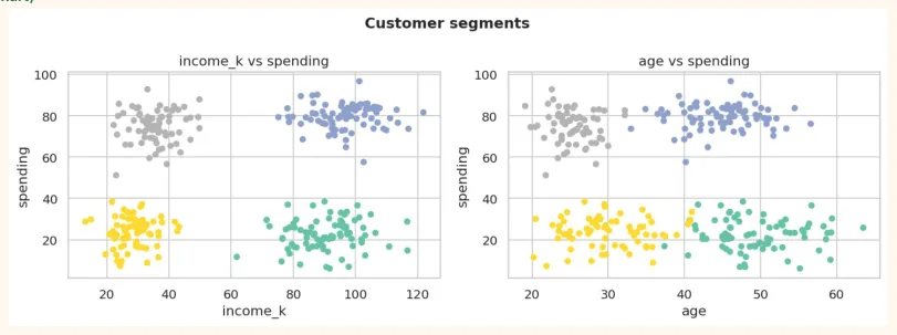
0 80 49.4 90.6 22.3 1 80 45.0 96.6 79.5 2 70 30.0 28.5 23.7 3 70 25.3 35.5 74.7 fig, axes = plt.subplots(1, 2, figsize=(11, 4)) for ax, (a, b) in zip(axes, [("income_k", "spending"), ("age", "spending")]): sc = ax.scatter(customers[a], customers[b], c=customers["segment"], cmap="Set2", s=22) ax.set_xlabel(a) ax.set_ylabel(b) ax.set_title(f"{a} vs {b}") fig.suptitle("Customer segments", fontsize=13, fontweight="bold") plt.tight_layout() plt.show() OUTPUT (chart)
Step 3: Name each segment and make a plan
The real benefit of clustering comes when we give each group a meaning . Looking at the profile table above (the average age, income and spending of each segment), write names in your own words. For example:
-
Young people with low income and high spending: installments and student discounts.
-
Rich and high spending: a loyalty program and premium products.
-
Rich but low spending: the biggest opportunity is here, offers that attract their attention.
-
Low income, low spending: cheap items, advertising at sale times.
REMEMBER
The names of the segments the data will not give, you will (domain knowledge). And if you change the K or the algorithm the segments can change, so treat the result as a helpful viewpoint , not as the final truth .
16.7 Hands-on
from sklearn.datasets import load_iris
iris_X = load_iris(as_frame=True).data
iris_y = load_iris().target                   # true species (not used in clustering)
iris_s = StandardScaler().fit_transform(iris_X)
lab = KMeans(n_clusters=3, n_init=10, random_state=0).fit_predict(iris_s) print(pd.crosstab(iris_y, lab, rownames=["True species"], colnames=["Cluster"])) OUTPUT Cluster 0 1 2 True species 0 0 50 0 1 39 0 11 2 14 0 36
-
K-Means on Iris: look at the crosstab above. Which species came out cleanly separate and which two species got mixed?
-
Elbow and silhouette: find both on Iris for K = 2 to 8. If the silhouette is highest at K = 2, why? (Hint: two species are very close to each other)
-
Hierarchical: make the dendrogram of Iris (ward linkage) and look at the crosstab for 3 clusters.
-
DBSCAN: on Iris (scaled) change eps from 0.3 to 1.0 and look at the number of clusters and noise points.
-
Customer segmentation: try K = 3 and K = 5 in 16.6 and see which segmentation is more useful for the business.
KEY TAKEAWAYS
-
Clustering is unsupervised: finding groups of similar things in data without labels. There is no correct answer, a human works out the meaning.
-
K-Means: pick K centroids, join points to the nearest centroid, make new centroids, repeat. Scaling is necessary, K has to be given.
-
To choose K use the Elbow method (inertia) and the Silhouette score (+1 better, 0 border).
-
Hierarchical: builds a tree (dendrogram), K is decided later by cutting. ward linkage is usually the best.
-
DBSCAN: makes clusters of dense areas, any shape, recognises noise itself (label -1). Needs eps and min_samples.
-
Customer segmentation is the most common use of clustering. Giving meaningful names to the segments is the data scientist's job.