Chapter 20: End-to-End ML Project and Case Study
MODULE 4 | WEEK 20
Chapter 20: End-to-End ML Project and Case Study
In the last 8 chapters we learned different pieces of ML. Now we join them all in one real, complete project: from the problem to the saved model . This is the same way it is done in real companies, and it can become the best project in your portfolio (GitHub).
20.1 Project: Titanic Survival Prediction
Question: who survived when the Titanic sank in 1912? From the passengers' information (class, sex, age, fare and so on), predict whether a passenger survived or not . This is binary classification .
Step 1: Problem definition
| Item | Decision |
|---|---|
| Problem | Binary classification (survived = 1 / 0) |
| Data | Seaborn's titanic dataset (891 passengers) |
| Measure of success | Accuracy + F1-score + ROC-AUC (the classes are about 62 / 38, so accuracy alone is not enough) |
| Baseline | A model that always says "died" (the most common class) |
| What we willnotdo | We will not touch the test set in tuning (leakage) |
Step 2: Data load and inspect
import numpy as np
import pandas as pd
import matplotlib.pyplot as plt
import seaborn as sns
titanic = sns.load_dataset("titanic")
print(titanic.shape)
print(titanic.dtypes.to_string())
print()
print("Missing values:")
print(titanic.isnull().sum()[titanic.isnull().sum() > 0].to_string())
OUTPUT
(891, 15)
survived          int64
pclass            int64
sex                 str
age             float64
sibsp             int64
parch             int64
fare            float64
embarked            str
class          category
who                 str
adult_male         bool
deck           category
embark_town         str
alive               str
alone              bool
Missing values:
age            177
embarked         2
deck           688
embark_town      2
In deck 688 values are empty (77%), in age 177, and in embarked and embark_town 2. We will drop deck (it would be wrong to fill in so many empty places).
Step 3: Spotting leakage and duplicate columns
In this dataset some columns are copies of each other , and one of them is the answer itself :
print(pd.crosstab(titanic["survived"], titanic["alive"])) print() print("Things like class vs pclass:") print(pd.crosstab(titanic["pclass"], titanic["class"])) OUTPUT alive no yes survived 0 549 0 1 0 342 Things like class vs pclass: class First Second Third pclass 1 216 0 0 2 0 184 0 3 0 0 491
-
alive ('yes' / 'no') is exactly like survived , meaning a copy of the target. Making it a feature is leakage : the model will give 100% accuracy but be useless on new data.
-
class is the same as pclass (only the name differs).
-
embark_town is the same as embarked . who and adult_male are made from sex and age. alone from sibsp and parch.
MOST IMPORTANT QUESTION
Any feature that was made because of the answer (target), or whose information is only available later is leakage. For every feature ask: "will this information be available at prediction time?"
cols = ["survived", "pclass", "sex", "age", "sibsp", "parch", "fare", "embarked"]
df = titanic[cols].copy()
print(df.shape)
print(df.head())
OUTPUT (891, 8) survived pclass sex age sibsp parch fare embarked 0 0 3 male 22.0 1 0 7.2500 S 1 1 1 female 38.0 1 0 71.2833 C 2 1 3 female 26.0 0 0 7.9250 S 3 1 1 female 35.0 1 0 53.1000 S 4 0 3 male 35.0 0 0 8.0500 S
Step 4: EDA (Exploratory Data Analysis)
print("Overall share who survived:", round(df["survived"].mean(), 3)) print() print(df.groupby("sex")["survived"].mean().round(3)) print() print(df.groupby("pclass")["survived"].mean().round(3)) OUTPUT Overall share who survived: 0.384 sex female 0.742 male 0.189 Name: survived, dtype: float64 pclass 1 0.630 2 0.473 3 0.242 Name: survived, dtype: float64 sns.set_theme(style="whitegrid") fig, axes = plt.subplots(1, 3, figsize=(13, 3.8)) sns.barplot(data=df, x="sex", y="survived", hue="sex", legend=False, ax=axes[0]) axes[0].set_title("Survival share by sex")
sns.barplot(data=df, x="pclass", y="survived", hue="sex", ax=axes[1])
axes[1].set_title("Class and sex")
sns.histplot(data=df, x="age", hue="survived", multiple="stack", bins=25, ax=axes[2]) axes[2].set_title("Age and survival") plt.tight_layout() plt.show() OUTPUT (chart)
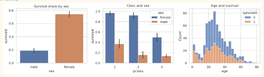
Observations: the share of women who survived was much higher than that of men. First class passengers survived more than second and third. Children (young age) had a higher chance of surviving. All this matches the "women and children first" rule of that time.
print("Share of missing age:", round(df["age"].isnull().mean(), 3))
print("Survived among those with missing age:", round(df[df["age"].isnull()]
["survived"].mean(), 3),
"| among the rest:", round(df[df["age"].notnull()]["survived"].mean(), 3))
OUTPUT
Share of missing age: 0.199 Survived among those with missing age: 0.294 | among the rest: 0.406 Among the passengers whose age was not known the share of survivors is lower. So "age being missing" is itself information . That is why along with imputation we will also keep a missing indicator (below).
Step 5: Feature Engineering
Making new and better features from the existing columns:
df["family_size"] = df["sibsp"] + df["parch"] + 1               # counting the person
themselves
df["is_alone"] = (df["family_size"] == 1).astype(int) print(df.groupby("family_size")["survived"].agg(["mean", "count"]).round(3)) OUTPUT
              mean  count
family_size
1 0.304 537 |
|---|
2 0.553 161 |
3 0.578 102 |
4 0.724 29 |
5 0.200 15 |
6 0.136 22 |
7 0.333 12 |
8 0.000 6 |
11 0.000 7 |
See: the survival share of passengers who were alone and of very big families is lower than that of families of medium size (2 to 4). This is a non-linear relationship , which trees and forests catch easily.
Step 6: Train/Test split and Baseline
from sklearn.model_selection import train_test_split
from sklearn.dummy import DummyClassifier
X = df.drop(columns="survived")
y = df["survived"]
X_train, X_test, y_train, y_test = train_test_split(X, y, test_size=0.2, random_state=42,
stratify=y)
print("Train:", X_train.shape, "| Test:", X_test.shape)
base = DummyClassifier(strategy="most_frequent").fit(X_train, y_train) print("Baseline accuracy:", round(base.score(X_test, y_test), 3)) OUTPUT
Train: (712, 9) | Test: (179, 9)
Baseline accuracy: 0.615
Step 7: Preprocessing Pipeline
Separate steps for numeric and categorical columns, all inside a ColumnTransformer , and with the model inside a Pipeline :
from sklearn.compose import ColumnTransformer
from sklearn.pipeline import make_pipeline
from sklearn.impute import SimpleImputer
from sklearn.preprocessing import StandardScaler, OneHotEncoder
numeric = ["age", "fare", "sibsp", "parch", "family_size", "is_alone"]
categorical = ["pclass", "sex", "embarked"]
num_pipe = make_pipeline(SimpleImputer(strategy="median", add_indicator=True),
StandardScaler())
cat_pipe = make_pipeline(SimpleImputer(strategy="most_frequent"),
OneHotEncoder(handle_unknown="ignore"))
preprocess = ColumnTransformer([("num", num_pipe, numeric), ("cat", cat_pipe, categorical)])
print(preprocess.fit_transform(X_train).shape, "(rows, new columns)")
OUTPUT
(712, 15) (rows, new columns)
-
add_indicator=True: for the columns in which values were missing, a 0/1 column is also made ("was this value missing?").
-
OneHotEncoder: turns pclass, sex, embarked into 0/1 columns. handle_unknown="ignore" saves from an error on a new category.
-
All the steps are inside the Pipeline, so there will be no leakage and they will be fitted separately in every CV fold.
Step 8: Comparing models (5-fold cross-validation)
from sklearn.model_selection import StratifiedKFold, cross_validate from sklearn.linear_model import LogisticRegression from sklearn.neighbors import KNeighborsClassifier from sklearn.svm import SVC from sklearn.ensemble import RandomForestClassifier, GradientBoostingClassifier models = { "Logistic Regression": LogisticRegression(max_iter=2000), "KNN": KNeighborsClassifier(n_neighbors=9), "SVM (rbf)": SVC(), "Random Forest": RandomForestClassifier(n_estimators=300, min_samples_leaf=3, random_state=0, n_jobs=-1), "Gradient Boosting": GradientBoostingClassifier(random_state=0), } cv = StratifiedKFold(n_splits=5, shuffle=True, random_state=42) rows = [] for name, model in models.items(): pipe = make_pipeline(preprocess, model) res = cross_validate(pipe, X_train, y_train, cv=cv, scoring=["accuracy", "f1", "roc_auc"]) rows.append((name, res["test_accuracy"].mean(), res["test_f1"].mean(), res["test_roc_auc"].mean())) compare = pd.DataFrame(rows, columns=["Model", "Accuracy", "F1", "ROCAUC"]).sort_values("ROC-AUC", ascending=False) print(compare.round(3).to_string(index=False)) OUTPUT Model Accuracy F1 ROC-AUC Gradient Boosting 0.820 0.751 0.887 Random Forest 0.815 0.741 0.878 Logistic Regression 0.803 0.733 0.856 SVM (rbf) 0.827 0.762 0.842 KNN 0.796 0.722 0.838
All the models are much better than the baseline (~0.62). The difference between several models is small , so it is necessary to compare a simple model with a complex model. We will tune a tree-based model (Random Forest or Gradient Boosting), because they learn non-linear relationships by themselves.
Step 9: Hyperparameter Tuning
from sklearn.model_selection import RandomizedSearchCV
from scipy.stats import randint
pipe = make_pipeline(preprocess, RandomForestClassifier(random_state=0, n_jobs=-1))
param_dist = {
    "randomforestclassifier__n_estimators": randint(100, 400),
    "randomforestclassifier__max_depth": randint(3, 12),
    "randomforestclassifier__min_samples_leaf": randint(1, 10),
"randomforestclassifier__max_features": ["sqrt", "log2", 0.5], } search = RandomizedSearchCV(pipe, param_dist, n_iter=25, cv=cv, scoring="roc_auc", random_state=0, n_jobs=-1) search.fit(X_train, y_train) print("Best CV ROC-AUC:", round(search.best_score_, 3)) print({k.split("__")[1]: (v if not isinstance(v, (np.integer, np.floating)) else v.item()) for k, v in search.best_params_.items()}) OUTPUT
Best CV ROC-AUC: 0.877
{'max_depth': 11, 'max_features': 'log2', 'min_samples_leaf': 4, 'n_estimators': 385}
Step 10: Final Evaluation (on the test set, only once)
from sklearn.metrics import (accuracy_score, precision_score, recall_score, f1_score, roc_auc_score, confusion_matrix, classification_report) best = search.best_estimator_ pred = best.predict(X_test) proba = best.predict_proba(X_test)[:, 1] print("Accuracy :", round(accuracy_score(y_test, pred), 3)) print("Precision:", round(precision_score(y_test, pred), 3)) print("Recall :", round(recall_score(y_test, pred), 3)) print("F1 :", round(f1_score(y_test, pred), 3)) print("ROC-AUC :", round(roc_auc_score(y_test, proba), 3)) print() print(classification_report(y_test, pred, target_names=["Died", "Survived"])) OUTPUT Accuracy : 0.799 Precision: 0.824 Recall : 0.609 F1 : 0.7 ROC-AUC : 0.841 precision recall f1-score support Died 0.79 0.92 0.85 110 Survived 0.82 0.61 0.70 69 accuracy 0.80 179 macro avg 0.81 0.76 0.77 179 weighted avg 0.80 0.80 0.79 179 from sklearn.metrics import ConfusionMatrixDisplay, roc_curve
fig, axes = plt.subplots(1, 2, figsize=(11, 4.2))
ConfusionMatrixDisplay.from_predictions(y_test, pred, display_labels=["Died", "Survived"],
cmap="Purples", ax=axes[0])
axes[0].set_title("Confusion Matrix (test set)")
fpr, tpr, _ = roc_curve(y_test, proba)
axes[1].plot(fpr, tpr, color="#A4457A", linewidth=2, label=f"Tuned Random Forest (AUC =
{roc_auc_score(y_test, proba):.3f})")
axes[1].plot([0, 1], [0, 1], "--", color="gray", label="Random guess")
axes[1].set_xlabel("False Positive Rate")
axes[1].set_ylabel("True Positive Rate")
axes[1].set_title("ROC curve")
axes[1].legend(loc="lower right")
plt.tight_layout()
plt.show()
OUTPUT (chart)
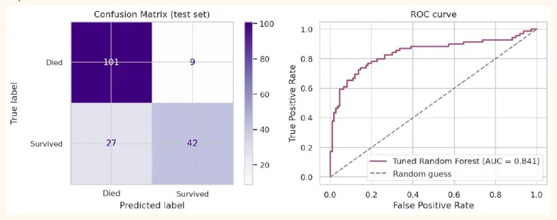
Here the recall (Survived) = 0.61 : of the passengers who really survived the model caught only 61%, while it caught 92% of the Died ones. So the model misses the "survivors" more. If our aim had been to identify the survivors, we would have had to lower the threshold (Chapter 14).
TEST VS CV
If the test score and CV score are close , it is a good sign that the model has not overfit. Here the CV ROC-AUC is 0.877 and the test ROC-AUC is 0.841, so there is a small difference . In a test set of only 179 rows the score moves 2 to 4 percent here and there, so this is normal. If the difference were very big (CV very good, test bad) we would suspect leakage or overfitting.
Step 11: Understanding the model: Permutation Importance
Which feature helped the most? Permutation importance : randomly shuffle the numbers of one feature and see how much the test score drops. The more it drops, the more important the feature. It works on any model , and reports on the original columns (from before preprocessing).
from sklearn.inspection import permutation_importance
imp = permutation_importance(best, X_test, y_test, n_repeats=15, random_state=0,
scoring="roc_auc", n_jobs=-1)
importance = pd.Series(imp.importances_mean, index=X_test.columns).sort_values(ascending=False) print(importance.round(3).to_string()) OUTPUT sex 0.235 pclass 0.028 age 0.019 fare 0.009 family_size 0.007 embarked 0.003 sibsp 0.002 parch 0.002 is_alone -0.003 importance.sort_values().plot(kind="barh", color="#6B5B95", figsize=(7, 4)) plt.title("Permutation importance (drop in ROC-AUC)") plt.xlabel("Importance") plt.show()
OUTPUT (chart)
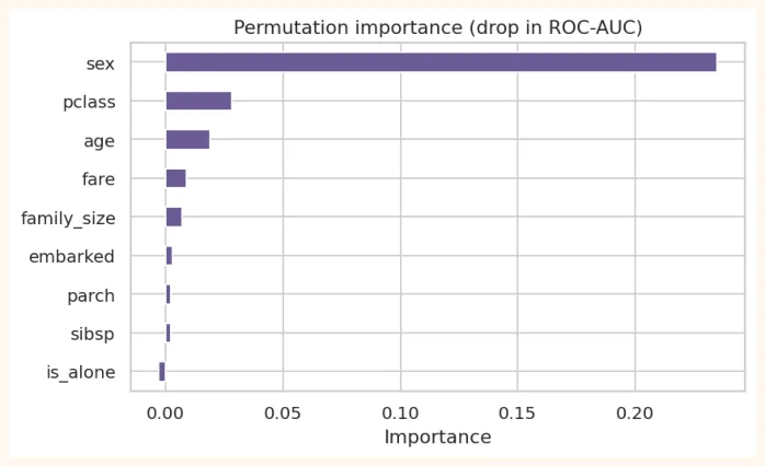
The effect of sex is many times larger than all the other features (0.235), with pclass and age far behind. This is the same as what we saw in the EDA. Negative importance (like is_alone) means that shuffling that feature made the score a little better, so that feature was no use to the model. Note: this tells what the model relied on , not the real cause. (The effect of sex was because of the "women and children first" rule of that time.)
Step 12: Error Analysis (where does the model go wrong?)
errors = X_test.copy() errors["actual"] = y_test errors["predicted"] = pred errors["prob_survive"] = proba.round(2) wrong = errors[errors["actual"] != errors["predicted"]] print("Wrong predictions:", len(wrong), "/", len(errors)) print("Share of errors by sex:") print(wrong["sex"].value_counts().to_string()) print() print(wrong.sort_values("prob_survive").head(5)[["pclass", "sex", "age", "fare", "actual", "prob_survive"]].to_string()) OUTPUT Wrong predictions: 36 / 179 Share of errors by sex: sex male 24 female 12 pclass sex age fare actual prob_survive 444 3 male NaN 8.1125 1 0.04 271 3 male 25.0 0.0000 1 0.06 570 2 male 62.0 10.5000 1 0.07 804 3 male 27.0 6.9750 1 0.07 17 2 male NaN 13.0000 1 0.08 Looking at the mistakes teaches a lot: does the model make more mistakes on a particular group (say men who survived, or women who did not)? In such unusual cases lies the hidden information that was not in the features, and the idea for the next experiment comes from there.
Step 13: Saving the model and a predict function
import joblib
joblib.dump(best, "titanic_model.joblib")
model = joblib.load("titanic_model.joblib")
def predict_survival(pclass, sex, age, sibsp, parch, fare, embarked): sample = pd.DataFrame([{ "pclass": pclass, "sex": sex, "age": age, "sibsp": sibsp, "parch": parch, "fare": fare, "embarked": embarked, "family_size": sibsp + parch + 1, "is_alone": int(sibsp + parch == 0), }]) p = model.predict_proba(sample)[0, 1] return round(float(p), 3), ("Survives" if p >= 0.5 else "Does not survive") print(predict_survival(pclass=1, sex="female", age=28, sibsp=0, parch=0, fare=80, embarked="S")) print(predict_survival(pclass=3, sex="male", age=35, sibsp=0, parch=0, fare=8, embarked="S")) OUTPUT (0.977, 'Survives') (0.167, 'Does not survive') Now this predict_survival function can be used in any app (FastAPI, Streamlit, or with the chatbot of the Docusaurus book). The complete way of deployment will come in Module 7 (MLOps).
Step 14: Writing the README / Report
When you put the project on GitHub, write these parts in the README.md :
-
Title and a 2-line summary: what the problem is and what the result was.
-
Data: source, size, columns, and which columns were removed and why (like alive, deck).
-
3 to 4 EDA charts and what you found from them.
-
Method: an outline of the pipeline (imputation, scaling, encoding), the models tried, tuning.
-
Result: a small table of metrics on the test set, a picture of the confusion matrix and ROC.
-
Limitations: a small dataset, data from 1912, the effect of chance, whether the model shows bias.
-
How to run: pip install -r requirements.txt and how to run the notebook.
-
Next step: more features, other models, deployment.
20.2 Mini Case Study: Regression (Diabetes progression)
Now let us look at a regression case, the same workflow in a smaller form. Goal: predict the progression of the disease after one year from 10 measurements. In this dataset the features are already scaled and there are no missing values, so our focus is on comparing models and the right measure .
from sklearn.datasets import load_diabetes
from sklearn.linear_model import Ridge, LassoCV
from sklearn.model_selection import cross_val_score, KFold
dX, dy = load_diabetes(return_X_y=True, as_frame=True)
dX_tr, dX_te, dy_tr, dy_te = train_test_split(dX, dy, test_size=0.2, random_state=42)
cv_r = KFold(n_splits=5, shuffle=True, random_state=0)
candidates = {
    "Baseline (average)": __import__("sklearn.dummy",
fromlist=["DummyRegressor"]).DummyRegressor(),
    "Linear Regression": __import__("sklearn.linear_model",
fromlist=["LinearRegression"]).LinearRegression(),
    "Ridge (alpha=0.1)": Ridge(alpha=0.1),
    "Random Forest": __import__("sklearn.ensemble",
fromlist=["RandomForestRegressor"]).RandomForestRegressor(n_estimators=300,
min_samples_leaf=5, random_state=0, n_jobs=-1),
    "Gradient Boosting": __import__("sklearn.ensemble",
fromlist=["GradientBoostingRegressor"]).GradientBoostingRegressor(n_estimators=100,
max_depth=2, learning_rate=0.05, random_state=0),
}
rows = []
for name, m in candidates.items(): r2 = cross_val_score(m, dX_tr, dy_tr, cv=cv_r, scoring="r2").mean() rmse = -cross_val_score(m, dX_tr, dy_tr, cv=cv_r, scoring="neg_root_mean_squared_error").mean() rows.append((name, r2, rmse)) print(pd.DataFrame(rows, columns=["Model", "CV R2", "CV RMSE"]).round(3).to_string(index=False)) OUTPUT Model CV R2 CV RMSE Baseline (average) -0.020 78.172 Linear Regression 0.494 54.944 Ridge (alpha=0.1) 0.494 54.965 Random Forest 0.411 59.146 Gradient Boosting 0.428 58.378 See: a simple linear model is equal to (or better than) the complex models. This dataset has a lot of noise and only 442 samples, so complex models give no benefit. Lesson: always start with a simple model and a baseline, and take a complex model only when it gives a clear improvement .
final = Ridge(alpha=0.1).fit(dX_tr, dy_tr) pred_d = final.predict(dX_te) from sklearn.metrics import r2_score, mean_absolute_error, mean_squared_error print("Test R2 :", round(r2_score(dy_te, pred_d), 3)) print("Test MAE :", round(mean_absolute_error(dy_te, pred_d), 1)) print("Test RMSE:", round(np.sqrt(mean_squared_error(dy_te, pred_d)), 1)) print("Std of the target (the baseline estimate):", round(dy_te.std(), 1)) OUTPUT Test R2 : 0.461 Test MAE : 43.0 Test RMSE: 53.4 Std of the target (the baseline estimate): 73.2 fig, axes = plt.subplots(1, 2, figsize=(11, 4)) axes[0].scatter(dy_te, pred_d, color="#6B5B95", alpha=0.7) lims = [dy_te.min(), dy_te.max()] axes[0].plot(lims, lims, "r--") axes[0].set_xlabel("Actual") axes[0].set_ylabel("Predicted") axes[0].set_title("Actual vs Predicted") axes[1].scatter(pred_d, dy_te - pred_d, color="#A4457A", alpha=0.7) axes[1].axhline(0, color="black", linestyle="--") axes[1].set_xlabel("Predicted") axes[1].set_ylabel("Residual") axes[1].set_title("Residuals") plt.tight_layout() plt.show() OUTPUT (chart)
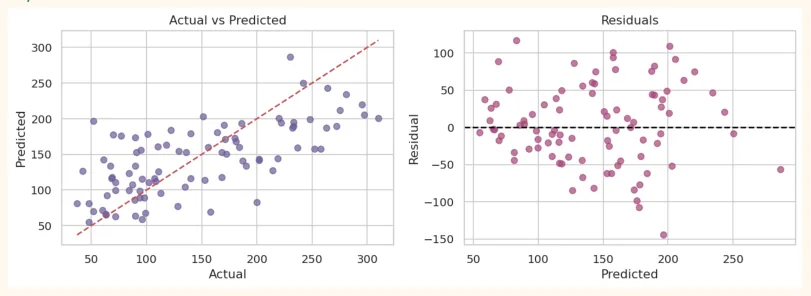
The model catches the trend of the target but there is also a lot of noise (R² is medium). This means that the progression of the disease cannot be predicted completely from only these 10 measurements, and a doctor's opinion is necessary for the real decision . Accepting the limits of the data is also a sign of a good data scientist.
20.3 Checklist of a complete ML Project
| Stage | Questions to ask |
|---|---|
| 1. Problem | Regression or classification? What is the measure of success? What is the cost of a mistake (FP or FN)? What is the baseline? |
| 2. Data | Where did it come from? How much? Is it representative? Issues of privacy and bias? |
| 3. Cleaning | Missing, duplicates, outliers, wrong types.Leakage columns? |
| 4. EDA | Distributions, relationships, imbalance. Anything strange? Does it match domain knowledge? |
| 5. Features | New features, encoding, scaling. Fit on train only. |
| 6. Modeling | Baseline, simple to complex models, cross-validation, tuning. |
| 7. Evaluation | The right metrics, the test set once, confusion matrix, ROC. Error analysis. |
| 8. Interpretation | Feature importance, coefficients, results that can be understood. |
| 9. Deployment | Save model + pipeline, predict function, app/API. Monitoring. |
| 10. Documentation | README, limitations, next step. Reproducible code (random_state, requirements). |
20.4 Hands-on
-
Rebuild: type out the whole Titanic project above yourself and run it in Colab (little copy-paste).
-
New feature: break age into bins (child, young, middle-aged, elderly) and see whether the test score changed.
-
Change the model: try Gradient Boosting in the tuning and compare it with Random Forest.
-
Threshold: instead of 0.5, put the threshold on proba at 0.4 and 0.6 and look at precision and recall.
-
Experience of leakage: put the 'alive' column in the features and see the score. How "good" does it come out, and why is it a deception?
-
Your own project: choose a small classification dataset from Kaggle or UCI (like heart disease, customer churn) and do everything from Step 1 to 14 and put it on GitHub with a README.
# Experience of leakage: when 'alive' is made a feature
leak = titanic[["pclass", "sex", "age", "fare", "alive", "survived"]].copy()
leak["alive"] = (leak["alive"] == "yes").astype(int)
leak["sex"] = (leak["sex"] == "female").astype(int)
leak["age"] = leak["age"].fillna(leak["age"].median())
Xl, yl = leak.drop(columns="survived"), leak["survived"]
Xl_tr, Xl_te, yl_tr, yl_te = train_test_split(Xl, yl, test_size=0.2, random_state=42,
stratify=yl)
print("Accuracy with leakage:", round(RandomForestClassifier(random_state=0).fit(Xl_tr,
yl_tr).score(Xl_te, yl_te), 3), "(fake 100%)")
OUTPUT
Accuracy with leakage: 1.0 (fake 100%)
KEY TAKEAWAYS
-
A complete ML project: problem, data, cleaning, EDA, features, split, pipeline, models, tuning, evaluation, interpretation, save, README.
-
Ask about every feature: will this information be available at prediction time? Otherwise it is leakage (like 'alive' = a copy of the target).
-
First a baseline, then simple to complex models, compare with cross-validation. A simple model is often enough.
-
ColumnTransformer + Pipeline gather numeric and categorical preprocessing in one place and prevent leakage.
-
Evaluate on the test set only once. Metrics: accuracy, precision, recall, F1, ROC-AUC, confusion matrix.
-
Permutation importance and error analysis help understand the model. Write the limitations and bias honestly.
-
Save the Pipeline with joblib and make a predict function. A good README makes the project worthy of a portfolio.