Chapter 15: Decision Trees and Random Forests
MODULE 4 | WEEK 15
Chapter 15: Decision Trees and Random Forests
The models so far (linear and logistic regression) worked on a straight line or a formula. A Decision Tree is a completely different way of thinking: it learns a series of questions from the data, which is exactly how a human makes a decision. Then a Random Forest combines very many trees into a very powerful model. These two algorithms are among the most widely used in the real world.
15.1 The Decision Tree idea
15.2 How does a tree choose a question? Impurity and Information Gain
At every node the tree chooses the question that splits the data into the cleanest (purest) parts. To measure "clean" we have a measure of impurity :
| Measure | Formula | Range | Meaning |
|---|---|---|---|
| Gini impurity(the sklearn | 1 - sum(p²) | 0 to 0.5 (2 classes) | 0 = perfectly pure (only one class), |
| default) | higher = mixed |
| Measure | Formula | Range | Meaning |
|---|---|---|---|
| Entropy | - sum(p x log2(p)) | 0 to 1 (2 classes) | 0 = pure, 1 = a 50-50 mix |
15.3 Overfitting: the biggest weakness of a tree
If a tree is allowed to grow without limits , it puts every training sample into its own leaf and gets 100% training accuracy, which means it memorizes the data (overfitting). On new data it does badly.
full = DecisionTreeClassifier(random_state=0).fit(X_train, y_train)
print("Full tree   -> depth:", full.get_depth(), "| leaves:", full.get_n_leaves(),
      "| train:", round(full.score(X_train, y_train), 3), "| test:",
round(full.score(X_test, y_test), 3))
small = DecisionTreeClassifier(max_depth=3, random_state=0).fit(X_train, y_train)
print("Depth = 3   -> depth:", small.get_depth(), "| leaves:", small.get_n_leaves(),
      "| train:", round(small.score(X_train, y_train), 3), "| test:",
round(small.score(X_test, y_test), 3))
OUTPUT
Full tree   -> depth: 5 | leaves: 8 | train: 1.0 | test: 0.967
Depth = 3   -> depth: 3 | leaves: 5 | train: 0.983 | test: 0.967
To avoid this we stop the tree (like pruning). The important hyperparameters:
| Hyperparameter | What it does |
|---|---|
| max_depth | The maximum depth of the tree |
| min_samples_split | The minimum number of samples needed to split a node |
| min_samples_leaf | The minimum number of samples in each leaf |
| max_leaf_nodes | The maximum number of leaves |
| max_features | How many features to choose from at each split |
| criterion | "gini" or "entropy" |
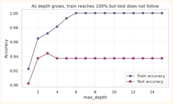
See what happens to the train and test scores when max_depth is changed (on the breast cancer data):
from sklearn.datasets import load_breast_cancer bc = load_breast_cancer(as_frame=True) Xb_train, Xb_test, yb_train, yb_test = train_test_split(bc.data, bc.target, test_size=0.25, random_state=1, stratify=bc.target) depths = range(1, 16) train_sc, test_sc = [], [] for d in depths: t = DecisionTreeClassifier(max_depth=d, random_state=0).fit(Xb_train, yb_train) train_sc.append(t.score(Xb_train, yb_train)) test_sc.append(t.score(Xb_test, yb_test)) print("Depth with the best test accuracy:", list(depths)[int(np.argmax(test_sc))], "| score:", round(max(test_sc), 3)) OUTPUT Depth with the best test accuracy: 3 | score: 0.944 plt.figure(figsize=(7.5, 4)) plt.plot(depths, train_sc, marker="o", color="#6B5B95", label="Train accuracy") plt.plot(depths, test_sc, marker="s", color="#A4457A", label="Test accuracy") plt.xlabel("max_depth") plt.ylabel("Accuracy") plt.title("As depth grows, train reaches 100% but test does not follow") plt.legend() plt.grid(alpha=0.3) plt.show() OUTPUT (chart)
Decision boundary: the tree thinks in boxes
On two features the tree divides its decision into rectangles (axis-parallel rectangles) , because every question is a threshold on one feature:
from sklearn.inspection import DecisionBoundaryDisplay
from sklearn.datasets import make_moons
Xm, ym = make_moons(n_samples=300, noise=0.3, random_state=0)
fig, axes = plt.subplots(1, 2, figsize=(10, 4))
for ax, depth, title in zip(axes, [3, None], ["max_depth = 3 (simple)", "No limit
(overfit)"]):
    m = DecisionTreeClassifier(max_depth=depth, random_state=0).fit(Xm, ym)
    DecisionBoundaryDisplay.from_estimator(m, Xm, ax=ax, alpha=0.4, cmap="coolwarm",
response_method="predict")
ax.scatter(Xm[:, 0], Xm[:, 1], c=ym, cmap="coolwarm", edgecolor="white", s=22) ax.set_title(title) plt.tight_layout() plt.show() OUTPUT (chart)
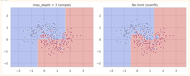
In the second chart the boundary has split into very curvy, tiny islands : the tree put even every noisy point into a separate class. This is the picture of overfitting.
15.4 Decision Tree Regression
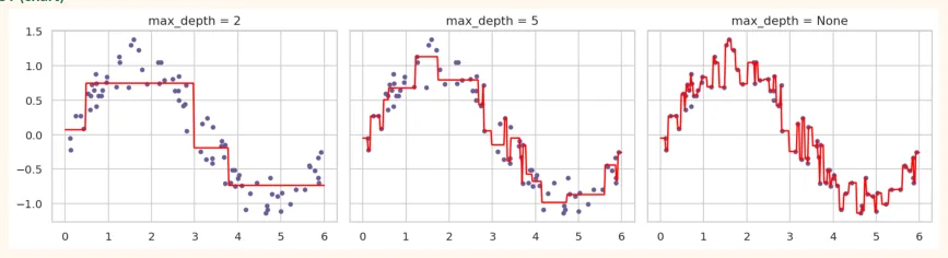
Trees predict not only classes but also numbers . A leaf holds the average of the samples in that part. The result looks like steps, not a straight line .
from sklearn.tree import DecisionTreeRegressor
np.random.seed(0)
xr = np.sort(np.random.uniform(0, 6, 80)).reshape(-1, 1)
yr = np.sin(xr).ravel() + np.random.normal(0, 0.2, 80)
xs = np.linspace(0, 6, 300).reshape(-1, 1)
fig, axes = plt.subplots(1, 3, figsize=(13, 3.5), sharey=True)
for ax, d in zip(axes, [2, 5, None]):
    m = DecisionTreeRegressor(max_depth=d, random_state=0).fit(xr, yr)
    ax.scatter(xr, yr, color="#6B5B95", s=14)
    ax.plot(xs, m.predict(xs), color="red")
    ax.set_title(f"max_depth = {d}")
plt.tight_layout()
plt.show()
OUTPUT (chart)
15.5 Feature Importance
The tree tells which feature helped the most in its decisions. The importance of each feature is measured by how much impurity was reduced by the splits it made (they all add up to 1).
t = DecisionTreeClassifier(max_depth=4, random_state=0).fit(Xb_train, yb_train) imp = pd.Series(t.feature_importances_, index=bc.data.columns).sort_values(ascending=False) print(imp.head(5).round(3)) OUTPUT worst concave points 0.751 worst area 0.138 mean texture 0.031 worst radius 0.030 worst texture 0.019 dtype: float64
15.6 Ensemble Learning and Random Forest
A single tree is weak and unreliable : a small change in the data produces a completely different tree (this is called high variance ). The idea of Ensemble Learning : combine very many weak models to make one strong model .
Bagging (Bootstrap Aggregating)
-
Take random samples again and again from the training data, with replacement (bootstrap): in each sample some rows appear 2-3 times and some do not appear at all.
-
Train a separate tree on each sample.
-
On new data take the vote of all trees (classification) or the average (regression).
Random Forest = Bagging + Random Features
Random Forest adds one more trick to bagging: at each split of each tree it is allowed to look at only a random part of the features ( max_features ). This way the trees do not all come out alike ( decorrelated ), and the ensemble is stronger.
| Item | What it is |
|---|---|
| n_estimators | How many trees (more = better and more stable, but slower). Usually 100 to 500 |
| Item | What it is |
|---|---|
| max_features | How many features to look at in each split (for classification usually sqrt(total features)) |
| max_depth, min_samples_leaf | The size of each tree (the same hyperparameters seen above) |
| bootstrap=True | Each tree trains on a different random sample |
| oob_score=True | Out-of-Bag score: free validation on the rows that did not come into the sample of a tree |
| n_jobs=-1 | Use all CPU cores (fast) |
| random_state | So that the result can be repeated |
from sklearn.ensemble import RandomForestClassifier
tree1 = DecisionTreeClassifier(random_state=0).fit(Xb_train, yb_train)
rf = RandomForestClassifier(n_estimators=200, oob_score=True, random_state=0, n_jobs=-
1).fit(Xb_train, yb_train)
print("Single Decision Tree test accuracy:", round(tree1.score(Xb_test, yb_test), 3)) print("Random Forest test accuracy :", round(rf.score(Xb_test, yb_test), 3)) print("Random Forest OOB score :", round(rf.oob_score_, 3)) OUTPUT
Single Decision Tree test accuracy: 0.937 Random Forest test accuracy : 0.944 Random Forest OOB score : 0.962 The OOB score is free validation: each tree has never seen ~37% of the data in its training, so the tree is tested on that. There is no need to create a separate validation set.
The effect of increasing the number of trees
for n in [1, 5, 20, 100, 400]: m = RandomForestClassifier(n_estimators=n, random_state=0, n_jobs=-1).fit(Xb_train, yb_train) print(f"n_estimators = {n:>3}: test accuracy = {m.score(Xb_test, yb_test):.3f}") OUTPUT n_estimators = 1: test accuracy = 0.895 n_estimators = 5: test accuracy = 0.944 n_estimators = 20: test accuracy = 0.951 n_estimators = 100: test accuracy = 0.944 n_estimators = 400: test accuracy = 0.944
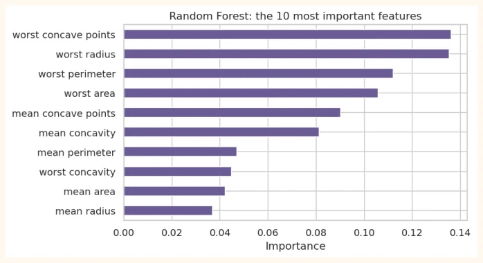
Feature importance of the Random Forest
imp = pd.Series(rf.feature_importances_, index=bc.data.columns).sort_values().tail(10)
plt.figure(figsize=(7, 4))
imp.plot(kind="barh", color="#6B5B95")
plt.title("Random Forest: the 10 most important features")
plt.xlabel("Importance")
plt.show()
OUTPUT (chart)
Random Forest regression
from sklearn.ensemble import RandomForestRegressor
from sklearn.datasets import load_diabetes
from sklearn.linear_model import LinearRegression
dX, dy = load_diabetes(return_X_y=True)
dXtr, dXte, dytr, dyte = train_test_split(dX, dy, test_size=0.2, random_state=42)
for name, m in [("Linear Regression", LinearRegression()), ("Decision Tree", DecisionTreeRegressor(random_state=0)), ("Random Forest", RandomForestRegressor(n_estimators=200, random_state=0, n_jobs=-1))]: m.fit(dXtr, dytr) print(f"{name:18s} test R2 = {m.score(dXte, dyte):.3f}") OUTPUT Linear Regression test R2 = 0.453 Decision Tree test R2 = -0.003 Random Forest test R2 = 0.420
Notice: the R² of the single Decision Tree is almost 0 (completely overfit), and the Random Forest is much better than that, but on this small and noisy dataset plain linear regression is still equal or better. Lesson: a complex model is not better on every dataset , always compare with a simple model.
15.7 Introduction to Boosting
In Bagging the trees are built in parallel and independently of each other. In Boosting the trees are built one after another (in sequence) , and each new tree focuses on correcting the mistakes of the previous trees .
15.8 Pros and cons of trees
| Pros of Decision Tree / Random Forest | Cons |
|---|---|
| Noneed for scaling | A single tree overfits quickly |
| Works with both numeric and categorical data | A Random Forest is hard to understand (like a black box) |
| Learnsnon-linearrelationships and feature interactions by itself | A big forest takes memory and time |
| Less affected by outliers | Cannot predict outside the range of the data (regression) |
| A single tree iseasy to understand | Problems with features that have very many categories |
| Gives feature importance | Less efficient than linear models on straight linear relationships |
15.9 Hands-on
A small workflow on seaborn's titanic dataset (who survived?):
import seaborn as sns titanic = sns.load_dataset("titanic") df = titanic[["survived", "pclass", "sex", "age", "sibsp", "parch", "fare"]].copy() print(df.shape, "| missing age:", df["age"].isnull().sum()) print(df["survived"].value_counts(normalize=True).round(3).to_dict()) OUTPUT
(891, 7) | missing age: 177
{0: 0.616, 1: 0.384}
df["age"] = df["age"].fillna(df["age"].median())
df["sex"] = (df["sex"] == "female").astype(int)           # female = 1
Xt, yt = df.drop(columns="survived"), df["survived"]
Xt_tr, Xt_te, yt_tr, yt_te = train_test_split(Xt, yt, test_size=0.2, random_state=42,
stratify=yt)
print("Baseline (call everyone 'died'):", round(1 - yt_te.mean(), 3)) for name, m in [("Decision Tree (depth 4)", DecisionTreeClassifier(max_depth=4, random_state=0)), ("Random Forest", RandomForestClassifier(n_estimators=300, min_samples_leaf=3, random_state=0, n_jobs=-1))]: m.fit(Xt_tr, yt_tr) print(f"{name:24s} test accuracy = {m.score(Xt_te, yt_te):.3f}") rf_t = RandomForestClassifier(n_estimators=300, min_samples_leaf=3, random_state=0, n_jobs=1).fit(Xt_tr, yt_tr) print(pd.Series(rf_t.feature_importances_, index=Xt.columns).sort_values(ascending=False).round(3)) OUTPUT
Baseline (call everyone 'died'): 0.615
Decision Tree (depth 4)  test accuracy = 0.777
Random Forest            test accuracy = 0.793
sex       0.382
fare      0.246
age       0.176
pclass    0.117
sibsp     0.044
parch     0.035
dtype: float64
-
See the tree: make a depth = 3 tree of Titanic with plot_tree. What is the question at the root?
-
Depth curve: plot the train and test accuracy for max_depth from 1 to 12.
-
min_samples_leaf: compare the test score at 1, 5, 20.
-
Forest: set n_estimators to 10, 100, 500 and look at the OOB score.
-
Thinking question: why is sex at the top of the feature importance? Does this mean gender was the cause , or only a sign?
KEY TAKEAWAYS
-
A Decision Tree learns a series of questions from data (if / else rules). Easy to understand, no scaling needed.
-
The split criterion: Gini or Entropy impurity; the question with the highest Information Gain is chosen.
-
A tree without limits overfits. Stop it with max_depth, min_samples_leaf and so on.
-
Ensemble: combining very many weak models. Bagging is parallel (bootstrap), Boosting is one after another (fixing mistakes).
-
Random Forest = bagging + random features at every split. Much better and more stable than a single tree. The OOB score is free validation.
-
Increasing n_estimators usually makes the result better or more stable. Control with max_features, max_depth, min_samples_leaf.
-
Feature importance tells what the model used more, not the cause. On table data Gradient Boosting is often the best.