Chapter 19: KNN, Model Optimization and Hyperparameter Tuning
MODULE 4 | WEEK 19
Chapter 19: KNN, Model Optimization and Hyperparameter Tuning
This chapter has two parts. First a simple but very easy-to-understand algorithm: K-Nearest Neighbors (KNN) . Then the most practical skill of ML: improving a model : cross-validation, learning curves, GridSearchCV , RandomizedSearchCV and Pipeline (so that there is no leakage).
19.1 K-Nearest Neighbors (KNN)
The idea of KNN is like how a human thinks: "tell me who I am by looking at my nearest neighbours ."
The algorithm
-
Decide K (say 5).
-
Compute the distance of the new point from all the points .
-
Pick the K nearest points.
-
Classification: the most common class among those K (vote). Regression: the average of those K.
How to measure distance?
| Measure | Formula | Meaning |
|---|---|---|
| Euclidean(default) | sqrt(sum((a - b)²)) | Straight-line (as the crow flies) distance |
| Manhattan | sum( | a - b |
| Minkowski | A general form of both (p = 1 Manhattan, p = 2 Euclidean) | The actual default of KNN |
a = np.array([1, 2]) b = np.array([4, 6]) print("Euclidean:", np.sqrt(((a - b) ** 2).sum())) # 5.0 print("Manhattan:", np.abs(a - b).sum()) # 7 OUTPUT Euclidean: 5.0 Manhattan: 7
KNN in sklearn
from sklearn.datasets import load_breast_cancer
from sklearn.model_selection import train_test_split
from sklearn.preprocessing import StandardScaler
from sklearn.pipeline import make_pipeline
bc = load_breast_cancer(as_frame=True)
X_train, X_test, y_train, y_test = train_test_split(bc.data, bc.target, test_size=0.25,
random_state=0, stratify=bc.target)
raw = KNeighborsClassifier(n_neighbors=5).fit(X_train, y_train) scaled = make_pipeline(StandardScaler(), KNeighborsClassifier(n_neighbors=5)).fit(X_train, y_train) print("Without scaling:", round(raw.score(X_test, y_test), 3)) print("With scaling :", round(scaled.score(X_test, y_test), 3)) OUTPUT Without scaling: 0.916 With scaling : 0.951 REMEMBER
KNN works on distance , so scaling is very necessary . The feature with big numbers dominates the distance.
Choosing K: bias-variance
-
K = 1: look only at the single nearest neighbour. The boundary is very curvy and picks up even noise → overfitting (high variance).
-
K very large: very many neighbours, the boundary becomes simple → underfitting (high bias). If K = the whole data, it always gives the most common class.
-
A usual start: K = 3 to 15 (odd numbers) , so that the vote is not tied. The best K is chosen by crossvalidation .
from sklearn.model_selection import cross_val_score
ks = range(1, 31)
cv_scores, train_scores = [], []
for k in ks:
    m = make_pipeline(StandardScaler(), KNeighborsClassifier(n_neighbors=k))
    cv_scores.append(cross_val_score(m, X_train, y_train, cv=5).mean())
    train_scores.append(m.fit(X_train, y_train).score(X_train, y_train))
best_k = list(ks)[int(np.argmax(cv_scores))]
plt.figure(figsize=(7.8, 4))
plt.plot(ks, train_scores, marker="o", markersize=3, color="#6B5B95", label="Train
accuracy")
plt.plot(ks, cv_scores, marker="s", markersize=3, color="#A4457A", label="Cross-validation
accuracy")
plt.axvline(best_k, color="gray", linestyle="--", label=f"Best K = {best_k}")
plt.xlabel("K (number of neighbours)")
plt.ylabel("Accuracy")
plt.title("The model gets simpler as K grows")
plt.legend()
plt.grid(alpha=0.3)
plt.show()
print("Best K:", best_k, "| CV accuracy:", round(max(cv_scores), 3))
OUTPUT (chart)
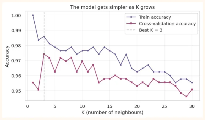
At K = 1 the train accuracy is 100% (every point is its own neighbour, memorizing). As K grows the train accuracy falls, while the CV accuracy first rises and then starts falling.
KNN Regression and weights
from sklearn.neighbors import KNeighborsRegressor
from sklearn.datasets import load_diabetes
dX, dy = load_diabetes(return_X_y=True)
dXtr, dXte, dytr, dyte = train_test_split(dX, dy, test_size=0.2, random_state=42)
for w in ["uniform", "distance"]:        # distance: more weight to the nearby ones
    m = KNeighborsRegressor(n_neighbors=10, weights=w).fit(dXtr, dytr)
    print(f"weights = {w:8s} test R2 = {m.score(dXte, dyte):.3f}")
OUTPUT
weights = uniform  test R2 = 0.412
weights = distance test R2 = 0.425
weights="distance" means the vote of a nearby neighbour counts for more (and that of a far one for less). Sometimes the result is better.
| Pros of KNN | Cons of KNN |
|---|---|
| Very simple and easy to understand | Prediction isslow(distance to all the data every time) |
| No training, new data is added easily | Scalingis necessary |
| Curvy boundaries form by themselves | Bad in many features (curse of dimensionality, Chapter 17) |
| Both classification and regression | Affected by irrelevant features and outliers; weak on imbalance |
19.2 Model Optimization: how to improve a model
Building a model and leaving it is not enough. It is necessary to learn the ways to improve it and the right way to evaluate it.
1) Cross-Validation (again, in depth)
In the earlier chapters we saw that we do not trust a single train/test split. K-Fold CV divides the data into K parts and does train/test K times. Stratified K-Fold keeps the share of the classes equal in every fold (always use this in classification).
from sklearn.model_selection import KFold, StratifiedKFold, cross_val_score, cross_validate
from sklearn.linear_model import LogisticRegression
model = make_pipeline(StandardScaler(), LogisticRegression(max_iter=2000))
skf = StratifiedKFold(n_splits=5, shuffle=True, random_state=42)
scores = cross_val_score(model, bc.data, bc.target, cv=skf) print("Accuracy:", scores.round(3), "-> average", scores.mean().round(3), "+/-", scores.std().round(3)) multi = cross_validate(model, bc.data, bc.target, cv=skf, scoring=["accuracy", "recall", "precision", "f1", "roc_auc"]) for m_name in ["accuracy", "recall", "precision", "f1", "roc_auc"]: print(f"{m_name:10s}: {multi['test_' + m_name].mean():.3f}") OUTPUT Accuracy: [0.974 0.947 0.965 0.991 0.991] -> average 0.974 +/- 0.017 accuracy : 0.974 recall : 0.992 precision : 0.968 f1 : 0.979 roc_auc : 0.995
2) Learning Curve: will more data help?
A learning curve is the graph of the train and validation score as the training data grows. It tells whether the model needs more data or a more complex model .
from sklearn.model_selection import learning_curve from sklearn.ensemble import RandomForestClassifier fig, axes = plt.subplots(1, 2, figsize=(11, 3.9), sharey=True) for ax, (name, est) in zip(axes, [("Logistic Regression (simple)", model), ("Random Forest (complex)", RandomForestClassifier(n_estimators=100, random_state=0))]): sizes, tr, va = learning_curve(est, bc.data, bc.target, cv=5, train_sizes=np.linspace(0.1, 1.0, 6), random_state=0) ax.plot(sizes, tr.mean(axis=1), marker="o", color="#6B5B95", label="Train") ax.plot(sizes, va.mean(axis=1), marker="s", color="#A4457A", label="Validation") ax.set_title(name) ax.set_xlabel("Training samples") ax.grid(alpha=0.3) axes[0].set_ylabel("Accuracy") axes[0].legend() plt.tight_layout() plt.show() OUTPUT (chart)
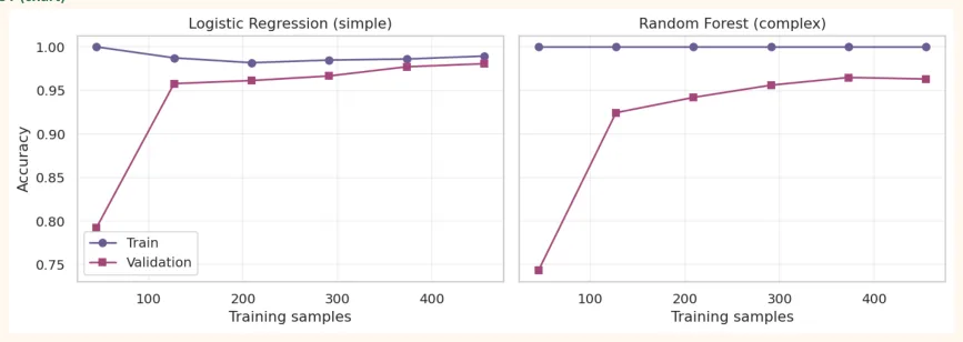
| What the graph looks like | Meaning | What to do |
|---|---|---|
| Train and validation bothlowand close | Underfitting(high bias) | A more complex model, better features, less regularization |
| Trainvery high, validation low, a big | Overfitting(high variance) | More data, a simpler model, regularization, fewer |
| gap | features | |
| Both close andgood, validation still rising | More data will help | Collect more data |
3) Validation Curve: the effect of one hyperparameter
from sklearn.model_selection import validation_curve
depths = [1, 2, 3, 5, 8, 12, 20] tr, va = validation_curve(RandomForestClassifier(n_estimators=50, random_state=0), bc.data, bc.target, param_name="max_depth", param_range=depths, cv=5) for d, t, v in zip(depths, tr.mean(axis=1), va.mean(axis=1)): print(f"max_depth = {d:>2}: train = {t:.3f} | validation = {v:.3f}") OUTPUT max_depth = 1: train = 0.938 | validation = 0.919 max_depth = 2: train = 0.963 | validation = 0.951 max_depth = 3: train = 0.978 | validation = 0.954 max_depth = 5: train = 0.994 | validation = 0.956 max_depth = 8: train = 0.999 | validation = 0.963 max_depth = 12: train = 1.000 | validation = 0.963 max_depth = 20: train = 1.000 | validation = 0.963
19.3 Hyperparameter Tuning
Hyperparameters are the settings we decide before training (K, C, gamma, max_depth, learning rate). The practical way to find the best combination is search :
GridSearchCV: try every possible combination
Looking at the results
results = pd.DataFrame(grid.cv_results_) cols = ["param_svc__C", "param_svc__kernel", "param_svc__gamma", "mean_test_score", "rank_test_score"] print(results[cols].sort_values("rank_test_score").head(5).round(3).to_string(index=False)) OUTPUT
 param_svc__C param_svc__kernel param_svc__gamma  mean_test_score  rank_test_score
          0.1            linear            scale            0.991                1
          0.1            linear             0.01            0.991                1
          1.0               rbf            scale            0.989                3
         10.0               rbf             0.01            0.985                4
          1.0            linear             0.01            0.983                5
RandomizedSearchCV: try random combinations (fast)
If there are many hyperparameters, grid search is very slow (10 values x 5 hyperparameters = 100,000 combinations!). RandomizedSearchCV tries n_iter random combinations, and from experience it usually gives the best result in less time.
from sklearn.model_selection import RandomizedSearchCV
from scipy.stats import randint, uniform
param_dist = {
    "n_estimators": randint(50, 300),
    "max_depth": randint(2, 20),
    "min_samples_leaf": randint(1, 10),
    "max_features": uniform(0.2, 0.7),          # between 0.2 and 0.9
}
rs = RandomizedSearchCV(RandomForestClassifier(random_state=0, n_jobs=-1), param_dist,
n_iter=15, cv=5,
scoring="f1", random_state=0, n_jobs=-1)
rs.fit(X_train, y_train)
print("Best combination:", {k: (float(round(v, 2)) if isinstance(v, float) else int(v)) for
k, v in rs.best_params_.items()})
print("CV f1:", round(rs.best_score_, 3), "| Test f1:", round(rs.score(X_test, y_test), 3)) OUTPUT
Best combination: {'max_depth': 16, 'max_features': 0.6, 'min_samples_leaf': 6, 'n_e...
CV f1: 0.968 | Test f1: 0.944
| GridSearchCV | RandomizedSearchCV | |
|---|---|---|
| Method | Tries every combination | Tries n_iter random combinations |
| When | Few hyperparameters and small value lists | Many hyperparameters, or continuous ranges |
| Time | More | You decide (n_iter) |
| Result | The very best inside the grid | Often close to the grid, in less time |
19.4 Pipeline: the complete way to avoid leakage
In Chapter 12 we saw that fitting the scaler on the whole data is leakage. Even during cross-validation, in every fold the scaler must be fitted only on the train part of that fold . A Pipeline takes care of this by itself.
# WRONG: scale the whole data first, then CV (the test fold's information went into the scaler) X_leaky = StandardScaler().fit_transform(bc.data) leaky = cross_val_score(KNeighborsClassifier(), X_leaky, bc.target, cv=5).mean() # RIGHT: the scaler inside a Pipeline, fitted separately in every fold clean = cross_val_score(make_pipeline(StandardScaler(), KNeighborsClassifier()), bc.data, bc.target, cv=5).mean() print("With leakage :", round(leaky, 4)) print("Pipeline (correct):", round(clean, 4)) OUTPUT With leakage : 0.9649 Pipeline (correct): 0.9649 On this dataset both scores came out the same (0.9649), because the data is big and clean and the effect on KNN is light. But this is not true for every dataset : with little data, many features, or steps like PCA/feature selection, leakage can make the result look falsely good , and this is dangerous because you never find out. So make it a habit: always a Pipeline.
A complete Pipeline: numeric + categorical columns
from sklearn.compose import ColumnTransformer from sklearn.impute import SimpleImputer from sklearn.preprocessing import OneHotEncoder from sklearn.ensemble import RandomForestClassifier df = pd.DataFrame({ "age": [25, 32, np.nan, 41, 29, 52, 36, 47, 33, 28, 60, 45], "income": [30, 45, 50, np.nan, 38, 90, 60, 75, 42, 35, 95, 80], "city": ["K", "L", "K", "I", "L", "K", "I", "L", "K", "I", "L", "K"], "bought": [0, 0, 0, 1, 0, 1, 1, 1, 0, 0, 1, 1], }) Xf, yf = df.drop(columns="bought"), df["bought"] prep = ColumnTransformer([ ("num", make_pipeline(SimpleImputer(strategy="median"), StandardScaler()), ["age", "income"]), ("cat", OneHotEncoder(handle_unknown="ignore"), ["city"]), ]) full = make_pipeline(prep, RandomForestClassifier(n_estimators=100, random_state=0)) print("CV accuracy:", cross_val_score(full, Xf, yf, cv=3).mean().round(3)) full.fit(Xf, yf) print("Prediction for the new customer:", full.predict(pd.DataFrame({"age": [38], "income": [70], "city": ["L"]}))) OUTPUT CV accuracy: 0.833 Prediction for the new customer: [1]
GridSearch with a Pipeline
The hyperparameters of a Pipeline are tuned by writing step_name__parameter (two underscores). This way even preprocessing can be included in the tuning.
pipe = make_pipeline(StandardScaler(), KNeighborsClassifier())
gs = GridSearchCV(pipe, {"kneighborsclassifier__n_neighbors": [3, 5, 7, 11, 15], "kneighborsclassifier__weights": ["uniform", "distance"]}, cv=5) gs.fit(X_train, y_train) print(gs.best_params_, "| CV:", round(gs.best_score_, 3), "| Test:", round(gs.score(X_test, y_test), 3)) OUTPUT
{'kneighborsclassifier__n_neighbors': 3, 'kneighborsclassifier__weights': 'uniform'...
19.5 Comparing models
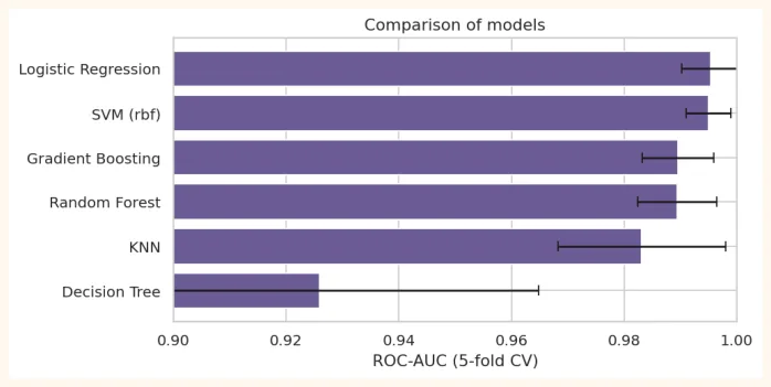
We try more than one model on the same cross-validation and make a table:
from sklearn.tree import DecisionTreeClassifier
from sklearn.ensemble import GradientBoostingClassifier
models = { "Logistic Regression": make_pipeline(StandardScaler(), LogisticRegression(max_iter=2000)), "KNN": make_pipeline(StandardScaler(), KNeighborsClassifier(n_neighbors=9)), "SVM (rbf)": make_pipeline(StandardScaler(), SVC()), "Decision Tree": DecisionTreeClassifier(max_depth=4, random_state=0), "Random Forest": RandomForestClassifier(n_estimators=200, random_state=0, n_jobs=-1), "Gradient Boosting": GradientBoostingClassifier(random_state=0), } rows = [] for name, m in models.items(): s = cross_val_score(m, bc.data, bc.target, cv=StratifiedKFold(5, shuffle=True, random_state=1), scoring="roc_auc") rows.append((name, s.mean(), s.std())) table = pd.DataFrame(rows, columns=["Model", "ROC-AUC mean", "std"]).sort_values("ROC-AUC mean", ascending=False) print(table.round(3).to_string(index=False)) OUTPUT Model ROC-AUC mean std Logistic Regression 0.995 0.005 SVM (rbf) 0.995 0.004 Gradient Boosting 0.990 0.006 Random Forest 0.989 0.007 KNN 0.983 0.015 Decision Tree 0.926 0.039 plt.figure(figsize=(7.5, 3.8)) plt.barh(table["Model"], table["ROC-AUC mean"], xerr=table["std"], color="#6B5B95", capsize=4) plt.xlim(0.9, 1.0) plt.gca().invert_yaxis() plt.xlabel("ROC-AUC (5-fold CV)") plt.title("Comparison of models") plt.show()
OUTPUT (chart)
19.6 Handling Class Imbalance
When one class is very small (fraud, disease), accuracy deceives (Chapter 14). Helpful methods: class_weight="balanced" , metrics like F1/recall/ROC-AUC/PR-AUC , and threshold tuning .
from sklearn.datasets import make_classification
from sklearn.metrics import recall_score, precision_score
Xi, yi = make_classification(n_samples=3000, n_features=10, weights=[0.95, 0.05],
random_state=0)
print("Class share:", np.bincount(yi) / len(yi))
Xi_tr, Xi_te, yi_tr, yi_te = train_test_split(Xi, yi, test_size=0.3, random_state=0,
stratify=yi)
for cw in [None, "balanced"]: m = LogisticRegression(class_weight=cw, max_iter=1000).fit(Xi_tr, yi_tr) p = m.predict(Xi_te) print(f"class_weight = {str(cw):9s} | accuracy = {m.score(Xi_te, yi_te):.3f} | recall = {recall_score(yi_te, p):.3f} | precision = {precision_score(yi_te, p):.3f}") OUTPUT
Class share: [0.946 0.054] class_weight = None | accuracy = 0.966 | recall = 0.449 | precision = 0.846 class_weight = balanced | accuracy = 0.884 | recall = 0.837 | precision = 0.299 After applying class_weight="balanced" , the recall (how many of the small class were caught) rose from 0.45 to 0.84, but the accuracy fell from 0.966 to 0.884 and the precision from 0.85 to 0.30 (very many false alarms). This is that same trade-off between precision and recall (Chapter 14). In a case like fraud, where missing one is costly, recall matters more, but false alarms have a cost too, so the balance of both is chosen according to the business. Other methods: oversampling (SMOTE, the imbalanced-learn library) and undersampling .
19.7 Saving and loading a model
After training we save the model to a file so that it does not have to be trained again and can be used in an app (FastAPI, Streamlit).
import joblib, os
best_model = gs.best_estimator_            # the whole Pipeline (scaler + KNN)
joblib.dump(best_model, "best_model.joblib")
print("File created:", os.path.exists("best_model.joblib"), "| size (KB):",
round(os.path.getsize("best_model.joblib") / 1024, 1))
loaded = joblib.load("best_model.joblib") print("Accuracy of the loaded model:", round(loaded.score(X_test, y_test), 3)) OUTPUT
File created: True | size (KB): 105.9
Accuracy of the loaded model: 0.951
19.8 Hands-on
-
KNN: on the wine dataset (load_wine) plot the CV accuracy for K = 1 to 25 and tell the best K. Also try it without scaling.
-
Distance: compare metric="manhattan" and "euclidean" in KNN.
-
Learning curve: make the learning curve of Logistic Regression and Random Forest on wine. Which one needs more data?
-
GridSearch: run GridSearchCV for a Random Forest (n_estimators, max_depth) on wine. Write down best_params_ and the test score.
-
Pipeline + save: make a Pipeline (StandardScaler + SVC) for wine, do GridSearch, and save and load the best model with joblib to check.
-
Thinking question: if a customer's data is very little (500 rows), which tuning strategy would you choose and why?
from sklearn.datasets import load_wine
wine = load_wine()
w_tr, w_te, wy_tr, wy_te = train_test_split(wine.data, wine.target, test_size=0.25, random_state=0, stratify=wine.target) for name, m in [("KNN (raw)", KNeighborsClassifier()), ("KNN (scaled)", make_pipeline(StandardScaler(), KNeighborsClassifier()))]: print(f"{name:14s} CV accuracy = {cross_val_score(m, w_tr, wy_tr, cv=5).mean():.3f}") OUTPUT KNN (raw) CV accuracy = 0.721 KNN (scaled) CV accuracy = 0.940
KEY TAKEAWAYS
-
KNN: the vote (classification) or average (regression) of the K nearest neighbours of a new point. A lazy learner, scaling is necessary.
-
K = 1 overfits (curvy), a very large K underfits. Choose K by cross-validation (usually an odd number).
-
Cross-validation (Stratified K-Fold) is a more trustworthy test than one split. TimeSeriesSplit for time series.
-
• The learning curve tells whether it is underfit, overfit, or more data will help. The validation curve shows the effect of one hyperparameter.
-
GridSearchCV tries every combination, RandomizedSearchCV random n_iter combinations. The test set is only for one final evaluation.
-
A Pipeline (preprocessing + model) prevents leakage and makes save/load easy. Tune with step__parameter.
-
Imbalanced data: class_weight, F1/recall/ROC-AUC. Save the model with joblib (the whole Pipeline).