Chapter 17: Dimensionality Reduction and PCA
MODULE 4 | WEEK 17
Chapter 17: Dimensionality Reduction and PCA
Real data often has very many columns (features) : thousands of pixels in a picture, hundreds of tests of a patient, thousands of words in a text. More features does not always mean better. Dimensionality Reduction reduces the number of columns and keeps the necessary information. The most famous method is PCA (Principal Component Analysis) .
17.1 The problem of too many features
The downsides of too many features
-
Danger of overfitting: with few samples and many features the model memorizes the data.
-
Slow training and more memory.
-
Distance-based algorithms (KNN, K-Means, SVM) get worse, because in many dimensions all points seem almost equally far.
-
Cannot visualize: we can only see 2D or 3D.
-
Many features are related to each other (correlated) , meaning the same information again and again.
import numpy as np
import pandas as pd
import matplotlib.pyplot as plt
# As dimensions grow, the difference between distances of random points disappears rng = np.random.RandomState(0) for d in [2, 10, 100, 1000]: pts = rng.uniform(0, 1, size=(200, d)) dists = np.sqrt(((pts[:1] - pts[1:]) ** 2).sum(axis=1)) print(f"{d:>4} dimensions: nearest / farthest = {dists.min() / dists.max():.2f}") OUTPUT
   2 dimensions: nearest / farthest = 0.04
  10 dimensions: nearest / farthest = 0.34
 100 dimensions: nearest / farthest = 0.77
1000 dimensions: nearest / farthest = 0.91
When the ratio gets close to 1 , the difference between "near" and "far" has vanished. This is why models like KNN do badly in many dimensions.
17.2 The PCA idea
PCA rotates the data onto new axes (principal components) such that:
-
The first axis (PC1) is the direction in which the data spreads the most (variance).
-
The second axis (PC2) is perpendicular (90 degrees) to the first and captures the most of the remaining spread, and so on.
-
Then we keep only the first few axes and drop the rest: fewer columns, most of the information kept.
OUTPUT (chart)
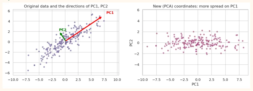
PC1 (red) lies in the direction of the longest spread of the data. If we drop PC2 and keep only PC1, 2 columns become 1 column, and most of the information is kept.
17.3 The steps of PCA (what happens inside)
-
Standardize: scale every feature (mean 0, std 1). PCA works on spread (variance), so scaling is necessary.
-
Compute the covariance matrix (how the features change together).
-
Find its eigenvectors (directions) and eigenvalues (how much spread in each direction).
-
Sort the eigenvalues from big to small. The direction with the biggest one is PC1 .
-
Pick the first k eigenvectors and project the data onto them. Now the data has k columns.
from sklearn.preprocessing import StandardScaler
# PCA by hand (on 2 features) and a comparison with sklearn
Z = StandardScaler().fit_transform(pts)
cov = np.cov(Z.T)
eigvals, eigvecs = np.linalg.eigh(cov)
order = np.argsort(eigvals)[::-1]
eigvals, eigvecs = eigvals[order], eigvecs[:, order]
print("Eigenvalues:", eigvals.round(3))
print("Share of the spread:", (eigvals / eigvals.sum()).round(3))
p = PCA(n_components=2).fit(Z) print("sklearn explained_variance_ratio_:", p.explained_variance_ratio_.round(3)) OUTPUT Eigenvalues: [1.876 0.134] Share of the spread: [0.933 0.067] sklearn explained_variance_ratio_: [0.933 0.067]
The answers of both methods are the same. That means sklearn's PCA does exactly this calculation inside.
17.4 PCA in scikit-learn: the Iris example
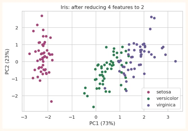
We reduce the 4 features of Iris to 2 and look at them in a 2D chart:
from sklearn.datasets import load_iris
from sklearn.pipeline import make_pipeline
iris = load_iris(as_frame=True)
X, y = iris.data, iris.target
print("Original shape:", X.shape)
pipe = make_pipeline(StandardScaler(), PCA(n_components=2))
X2 = pipe.fit_transform(X)
print("Shape after PCA:", X2.shape)
pca_iris = pipe[-1]
print("Spread of each component:", pca_iris.explained_variance_ratio_.round(3))
print("Sum of both:", pca_iris.explained_variance_ratio_.sum().round(3))
OUTPUT
Original shape: (150, 4)
Shape after PCA: (150, 2)
Spread of each component: [0.73  0.229]
Sum of both: 0.958
Just 2 components captured about 96% of the spread, meaning that by turning 4 columns into 2 we lost only 4% of the information. Now we can plot this:
plt.figure(figsize=(7, 4.4)) for cls, color in zip([0, 1, 2], ["#A4457A", "#2F7D4F", "#6B5B95"]): mask = (y == cls).values plt.scatter(X2[mask, 0], X2[mask, 1], color=color, label=iris.target_names[cls], s=28) plt.xlabel(f"PC1 ({pca_iris.explained_variance_ratio_[0] * 100:.0f}%)") plt.ylabel(f"PC2 ({pca_iris.explained_variance_ratio_[1] * 100:.0f}%)") plt.title("Iris: after reducing 4 features to 2") plt.legend() plt.show() OUTPUT (chart)
What are the components? (loadings)
Each principal component is a combination of the original features. components_ tells how much weight each feature has in it:
loadings = pd.DataFrame(pca_iris.components_, columns=X.columns, index=["PC1", "PC2"])
print(loadings.round(2))
OUTPUT
     sepal length (cm)  sepal width (cm)  petal length (cm)  \
PC1               0.52             -0.27               0.58
PC2               0.38              0.92               0.02
     petal width (cm)
PC1              0.56
PC2              0.07
In PC1 the weights of petal length, petal width and sepal length are positive and large, meaning PC1 is a kind of "flower size" . This is why the species look clearly separated along PC1 in the chart.
17.5 How many components to choose?
The Explained variance ratio tells how much spread (information) each component captured. Two ways:
- Cumulative variance: keep as many components as needed so that the total spread reaches 95% (or 90%).
• Scree plot: the graph of variance; stop where the elbow appears.
full = make_pipeline(StandardScaler(), PCA()).fit(X)       # all components
ratios = full[-1].explained_variance_ratio_
print("Each component:", ratios.round(3))
print("Cumulative   :", ratios.cumsum().round(3))
OUTPUT
Each component: [0.73  0.229 0.037 0.005]
Cumulative   : [0.73  0.958 0.995 1.   ]
You can also tell PCA directly that you want 95% variance and it picks the number of components itself:
auto = make_pipeline(StandardScaler(), PCA(n_components=0.95)).fit(X) print("Components for 95%:", auto[-1].n_components_) OUTPUT Components for 95%: 2
17.6 PCA on bigger data: Digits (64 features)
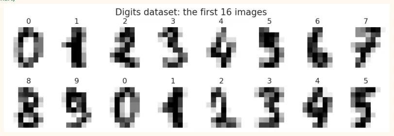
The Digits dataset: 1,797 images of handwritten digits from 0 to 9, each image is 8 x 8 = 64 pixels (that is, 64 features).
from sklearn.datasets import load_digits
digits = load_digits() Xd, yd = digits.data, digits.target print(Xd.shape, "| pixel range:", Xd.min(), "to", Xd.max()) OUTPUT
(1797, 64) | pixel range: 0.0 to 16.0 fig, axes = plt.subplots(2, 8, figsize=(11, 3.2)) for i, ax in enumerate(axes.ravel()): ax.imshow(digits.images[i], cmap="gray_r") ax.set_title(digits.target[i]) ax.axis("off") plt.suptitle("Digits dataset: the first 16 images") plt.show() OUTPUT (chart)
Reducing 64 columns to 2 and looking at them
from sklearn.decomposition import PCA
Xd2 = PCA(n_components=2).fit_transform(Xd)
plt.figure(figsize=(7.5, 5.2))
sc = plt.scatter(Xd2[:, 0], Xd2[:, 1], c=yd, cmap="tab10", s=10)
plt.colorbar(sc, label="Digit")
plt.xlabel("PC1")
plt.ylabel("PC2")
plt.title("Digits: 64 dimensions in 2D")
plt.show()
OUTPUT (chart)
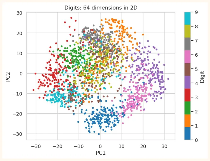
Even in just 2 axes most digits appear in separate groups (with some overlap). This is a wonderful way to show 64-dimensional data in one picture.
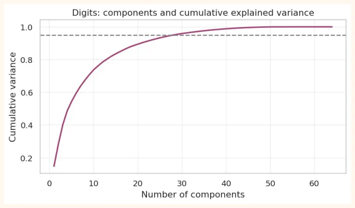
pca_full = PCA().fit(Xd) cum = pca_full.explained_variance_ratio_.cumsum() for target in [0.80, 0.90, 0.95, 0.99]: print(f"Components for {int(target * 100)}% variance: {int(np.argmax(cum >= target)) + 1}") OUTPUT Components for 80% variance: 13 Components for 90% variance: 21 Components for 95% variance: 29 Components for 99% variance: 41 plt.figure(figsize=(7.5, 3.8)) plt.plot(range(1, 65), cum, color="#A4457A", linewidth=2) plt.axhline(0.95, color="gray", linestyle="--") plt.title("Digits: components and cumulative explained variance") plt.xlabel("Number of components") plt.ylabel("Cumulative variance") plt.grid(alpha=0.3) plt.show()
OUTPUT (chart)
17.7 Compression and Reconstruction with PCA
PCA can make data smaller , and then bring it back (inverse_transform) to full size, but some information will be lost. See at how many components the digit can still be recognised:
sample = Xd[:6]
fig, axes = plt.subplots(5, 6, figsize=(8.5, 7.5))
rows = [("Original (64)", None), ("30 comp.", 30), ("15 comp.", 15), ("8 comp.", 8), ("3
comp.", 3)]
for r, (name, n) in enumerate(rows):
    if n is None:
        recon = sample
    else:
        p = PCA(n_components=n).fit(Xd)
        recon = p.inverse_transform(p.transform(sample))
    for c in range(6):
        axes[r, c].imshow(recon[c].reshape(8, 8), cmap="gray_r")
        axes[r, c].axis("off")
    axes[r, 0].set_title(name, loc="left", fontsize=9)
plt.tight_layout()
plt.show()
OUTPUT (chart)
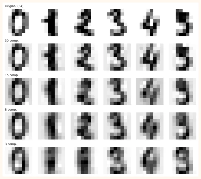
At 30 components the picture is almost like the original (less than half the columns), at 15 it is still readable, and at 3 it is very blurry. This shows that most of the information in the data lies in just a few directions.
17.8 Using PCA before a model
PCA can be placed in a Pipeline before a model as a preprocessing step . This makes training faster and sometimes the model better (less overfit).
from sklearn.model_selection import cross_val_score, train_test_split
from sklearn.linear_model import LogisticRegression
from sklearn.neighbors import KNeighborsClassifier
import time
Xtr, Xte, ytr, yte = train_test_split(Xd, yd, test_size=0.25, random_state=0, stratify=yd) for name, pipe in [ ("KNN, 64 features ", make_pipeline(StandardScaler(), KNeighborsClassifier())), ("PCA(95%) + KNN ", make_pipeline(StandardScaler(), PCA(n_components=0.95), KNeighborsClassifier())), ("PCA(10) + KNN ", make_pipeline(StandardScaler(), PCA(n_components=10), KNeighborsClassifier())), ]: t = time.time() pipe.fit(Xtr, ytr) acc = pipe.score(Xte, yte) print(f"{name} accuracy = {acc:.3f} | time = {time.time() - t:.3f}s") OUTPUT KNN, 64 features accuracy = 0.973 | time = 0.010s PCA(95%) + KNN accuracy = 0.969 | time = 0.013s PCA(10) + KNN accuracy = 0.916 | time = 0.016s
REMEMBER
The fit of PCA too must be on the train data only (to avoid leakage). Placing it in a Pipeline does this automatically, and in cross-validation it is fitted separately in every fold.
17.9 Limits of PCA and a glimpse of t-SNE
| Pros of PCA | Limits of PCA |
|---|---|
| Fast, simple, strong | Captures only**straight (linear)**relationships |
| Removes correlated features | The components are hard to interpret (combinations of original features) |
| Visualization and compression | Depends heavily on scaling |
| Helps reduce noise | More spread is not always moreusefulinformation |
| Less overfitting | Outliers distort the spread |
When the data has a curvy (non-linear) structure, PCA is weak. There algorithms like t-SNE and UMAP give better visualization . t-SNE is only for looking (it cannot transform new data), and you can trust its small distances, not the big ones.
from sklearn.manifold import TSNE
tsne = TSNE(n_components=2, random_state=0, init="pca",
perplexity=30).fit_transform(Xd[:1000])
plt.figure(figsize=(7.5, 5.2))
sc = plt.scatter(tsne[:, 0], tsne[:, 1], c=yd[:1000], cmap="tab10", s=10)
plt.colorbar(sc, label="Digit")
plt.title("t-SNE: a better picture of the digit groups (1000 samples)") plt.show() OUTPUT (chart)
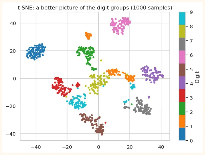
In t-SNE the digits appear as more clearly separate groups than in PCA. But t-SNE is slow , and its axes have no direct meaning.
17.10 Hands-on
from sklearn.datasets import load_breast_cancer
bc = load_breast_cancer(as_frame=True)
Xb, yb = bc.data, bc.target
cumb = make_pipeline(StandardScaler(), PCA()).fit(Xb)[-1].explained_variance_ratio_.cumsum()
print("Breast cancer: 30 features. Components for 95% variance:", int(np.argmax(cumb >=
0.95)) + 1)
OUTPUT
Breast cancer: 30 features. Components for 95% variance: 10
-
Breast cancer: apply PCA on the 30 features, make a scatter plot with 2 components (colour = malignant / benign). Do the two classes look separate?
-
Scree plot: plot the explained variance for breast cancer and find the elbow.
-
Pipeline: run LogisticRegression on breast cancer with (a) all 30 features, (b) PCA(5), (c) PCA(2) and compare the test accuracy.
-
Loadings: which 3 features have the most weight in PC1?
-
Thinking question: if you had to explain the model's decisions to a doctor, why would it be hard to use features after PCA?
Xb_tr, Xb_te, yb_tr, yb_te = train_test_split(Xb, yb, test_size=0.25, random_state=0,
stratify=yb)
for name, steps in [("30 features", [StandardScaler(), LogisticRegression(max_iter=2000)]),
                    ("PCA(5)     ", [StandardScaler(), PCA(5),
LogisticRegression(max_iter=2000)]),
                    ("PCA(2)     ", [StandardScaler(), PCA(2),
LogisticRegression(max_iter=2000)])]:
    m = make_pipeline(*steps).fit(Xb_tr, yb_tr)
    print(f"{name} test accuracy = {m.score(Xb_te, yb_te):.3f}")
OUTPUT
30 features test accuracy = 0.958
PCA(5)      test accuracy = 0.965
PCA(2)      test accuracy = 0.923
KEY TAKEAWAYS
-
The downsides of too many features: overfitting, slow training, distance-based algorithms getting worse (curse of dimensionality), being unable to visualize.
-
PCA makes new axes (principal components) that capture the most spread (variance). PC1 is the most important, PC2 is perpendicular to it.
-
Steps: standardize, covariance, eigenvectors and eigenvalues, pick the top k and project. Scaling is necessary.
-
explained_variance_ratio_ tells how much information each component captured. PCA(n_components=0.95) picks the number by itself.
-
With PCA, visualization (Iris 4D to 2D, Digits 64D to 2D), compression and reconstruction (inverse_transform) are possible.
-
Put PCA in a Pipeline so that fit is on train only. PCA captures only linear structure; for non-linear use t- SNE/UMAP (visualization only).