Chapter 13: Linear Regression Deep Dive, Gradient Descent and Regularization
MODULE 4 | WEEK 13
Chapter 13: Linear Regression Deep Dive, Gradient Descent and Regularization
In Module 3 we looked at linear regression from the statistics point of view. Now we look at it from the ML point of view : how does the model learn ? The answer is Gradient Descent , the very same idea that is used to train neural networks. Then we will learn Regularization (L1, L2) , which protects the model from overfitting.
13.1 Cost Function: the measure of the model's error
The linear regression line is y = w x + b (here w is the slope and b the intercept). We need the values of w and b for which the model's error is the smallest. To measure the error we build a cost function (or loss function). In linear regression this is usually MSE (Mean Squared Error) :
J(w, b) = (1/n) x sum( (prediction - actual)² )
13.2 Gradient Descent
Gradient means the slope (of the cost) : it tells whether increasing a parameter will increase or decrease the cost. We change the parameter a little in the opposite direction of the slope .
w = w - alpha x (dJ/dw) and b = b - alpha x (dJ/db)
-
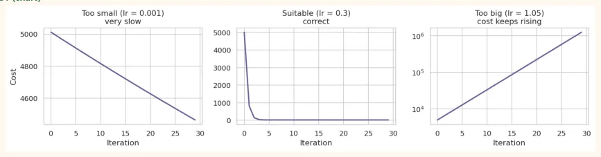
alpha (learning rate): the size of the step. If it is very small you will arrive slowly; if it is very big you will leap over the valley.
-
dJ/dw: how much the cost changes when w changes (derivative / slope).
-
This process is repeated (iterations) until the cost stops decreasing.
The derivatives for MSE are these (n = number of samples, error = prediction - actual):
-
dJ/dw = (2/n) x sum(error x x)
-
dJ/db = (2/n) x sum(error)
Gradient Descent by hand (in NumPy)
First we scale x (we explain the reason below), then run the loop:
x = (hours - hours.mean()) / hours.std()       # scaled feature
y = marks
w, b = 0.0, 0.0           # both start at 0
lr = 0.1                  # learning rate
n = len(x)
history = []
for i in range(100):
    pred = w * x + b
    error = pred - y
    history.append((error ** 2).mean())        # record the cost
    dw = (2 / n) * (error * x).sum()
    db = (2 / n) * error.sum()
    w = w - lr * dw
    b = b - lr * db
    if i in (0, 1, 5, 20, 99):
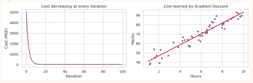
print(f"iteration {i + 1:>3}: w = {w:6.2f}, b = {b:6.2f}, cost = {history[1]:8.2f}") OUTPUT iteration 1: w = 2.86, b = 13.84, cost = 5012.34 iteration 2: w = 5.14, b = 24.91, cost = 3215.60 iteration 6: w = 10.54, b = 51.05, cost = 557.29 iteration 21: w = 14.15, b = 68.55, cost = 22.05 iteration 100: w = 14.28, b = 69.19, cost = 21.39 The cost is falling at every iteration and w, b are settling down. Now we bring these parameters back to the original scale and compare them with polyfit (the correct answer):
slope = w / hours.std() intercept = b - slope * hours.mean() print("Gradient Descent:", round(slope, 3), round(intercept, 3)) b1, b0 = np.polyfit(hours, marks, 1) print("polyfit (correct):", round(b1, 3), round(b0, 3)) OUTPUT Gradient Descent: 5.829 35.135 polyfit (correct): 5.829 35.135 fig, axes = plt.subplots(1, 2, figsize=(11, 3.6)) axes[0].plot(history, color="#A4457A", linewidth=2) axes[0].set_title("Cost decreasing at every iteration") axes[0].set_xlabel("Iteration") axes[0].set_ylabel("Cost (MSE)") axes[1].scatter(hours, marks, color="#6B5B95", s=18) xs = np.linspace(1, 10, 50) axes[1].plot(xs, intercept + slope * xs, color="red", linewidth=2) axes[1].set_title("Line learned by Gradient Descent") axes[1].set_xlabel("Hours") axes[1].set_ylabel("Marks") plt.tight_layout() plt.show() OUTPUT (chart)
The effect of the learning rate
def gradient_descent(x, y, lr, iters=60):
    w = b = 0.0
    n = len(x)
    costs = []
    for _ in range(iters):
        error = w * x + b - y
        costs.append((error ** 2).mean())
        w -= lr * (2 / n) * (error * x).sum()
        b -= lr * (2 / n) * error.sum()
    return costs
for lr in [0.001, 0.3, 1.05]:
c = gradient_descent(x, y, lr) print(f"lr = {lr:>5}: starting cost = {c[0]:8.1f} | final cost = {c[-1]:.3g}") OUTPUT lr = 0.001: starting cost = 5012.3 | final cost = 3.96e+03 lr = 0.3: starting cost = 5012.3 | final cost = 21.4 lr = 1.05: starting cost = 5012.3 | final cost = 3.82e+08 fig, axes = plt.subplots(1, 3, figsize=(13, 3.4)) for ax, lr, title in zip(axes, [0.001, 0.3, 1.05], ["Too small (lr = 0.001)\nvery slow", "Suitable (lr = 0.3)\ ncorrect", "Too big (lr = 1.05)\ncost keeps rising"]): ax.plot(gradient_descent(x, y, lr, iters=30), color="#6B5B95", linewidth=2) ax.set_title(title) ax.set_xlabel("Iteration") axes[0].set_ylabel("Cost") axes[2].set_yscale("log") plt.tight_layout() plt.show() OUTPUT (chart)
PRACTICAL TIP
The learning rate is one of the most important hyperparameters. A common start: try 0.1, 0.01, 0.001 and look at the cost graph. If the cost is rising , lower the learning rate.
Why is feature scaling important for gradient descent?
If the scales of the features are very different (one from 0 to 1, another from 0 to 100,000), the cost "bowl" turns into a long narrow channel , and gradient descent zig-zags inside it and arrives very slowly (or diverges). Scaling makes the bowl round , and it goes straight down.
# Same learning rate (0.01), same iterations, but scaled vs unscaled x
print("Scaled x   :", round(gradient_descent(x, y, 0.01, iters=200)[-1], 2))
print("Unscaled x :", round(gradient_descent(hours, y, 0.01, iters=200)[-1], 2))
print("Lowest possible cost:", round(((np.polyval(np.polyfit(hours, marks, 1), hours) -
marks) ** 2).mean(), 2))
OUTPUT Scaled x : 23.0 Unscaled x : 73.82 Lowest possible cost: 21.39
The cost with scaled data came close to the lowest possible cost, while the unscaled one is still far away.
Types of Gradient Descent
| Type | How much data at each step | Characteristics |
|---|---|---|
| Batch | Thewholetraining data | Accurate and stable, but slow on big data |
| Type | How much data at each step | Characteristics |
|---|---|---|
| Stochastic (SGD) | Onesample | Fast, noisy (the line wobbles), good for big data |
| Mini-batch | Small batches (like 32 or 64 samples) | The golden middle of both,the most common in deep learning |
from sklearn.linear_model import SGDRegressor
sgd = SGDRegressor(max_iter=2000, tol=1e-4, random_state=0) sgd.fit(x.reshape(-1, 1), y) print("SGD slope, intercept (on scaled x):", round(sgd.coef_[0], 2), round(sgd.intercept_[0], 2)) print("Our hand-made one: ", round(w, 2), round(b, 2)) OUTPUT SGD slope, intercept (on scaled x): 14.28 69.17 Our hand-made one: 14.28 69.19
Normal Equation: a direct solution without gradient descent
Linear regression also has a formula that gives the best w directly: w = (X^T X)^(-1) X^T y . Scikit-learn's LinearRegression generally uses this (or something like it).
| Normal Equation | Gradient Descent | |
|---|---|---|
| Learning rate | Not needed | Has to be chosen |
| Iterations | None, done in one go | Many |
| Many features (hundreds of | Slow(matrix inverse is expensive) | Fast |
| thousands) | ||
| Very many samples | Can be slow | Easy with mini-batch |
| Works on | Only linear regression | Everything(logistic, neural networks...) |
This is why gradient descent is so important: it is the basic way of training not just linear regression, but every ML and deep learning model .
13.3 Multiple Linear Regression (with scikit-learn)
Now a real dataset: Diabetes (442 patients, 10 measurements such as age, BMI, blood pressure, and the target: a measure of disease progression after one year). The features of this data are already scaled.
from sklearn.datasets import load_diabetes
from sklearn.model_selection import train_test_split
from sklearn.linear_model import LinearRegression
from sklearn.metrics import mean_squared_error, r2_score
data = load_diabetes(as_frame=True) X, y = data.data, data.target print(X.shape) print(X.columns.tolist()) X_train, X_test, y_train, y_test = train_test_split(X, y, test_size=0.2, random_state=42) lin = LinearRegression().fit(X_train, y_train) pred = lin.predict(X_test) print("Test R2 :", round(r2_score(y_test, pred), 3)) print("Test RMSE:", round(np.sqrt(mean_squared_error(y_test, pred)), 2)) print(pd.Series(lin.coef_, index=X.columns).round(1)) OUTPUT (442, 10) ['age', 'sex', 'bmi', 'bp', 's1', 's2', 's3', 's4', 's5', 's6']
Test R2  : 0.453
Test RMSE: 53.85
age     37.9
sex   -242.0
bmi    542.4
bp     347.7
s1    -931.5
s2     518.1
s3     163.4
s4     275.3
s5     736.2
s6      48.7
dtype: float64
Notice: some coefficients are very big (like those of s1 and s2 ), which raises the suspicion that these features are strongly related to each other. When this happens the model becomes very sensitive , and this is exactly where regularization helps.
13.4 Polynomial Regression and Overfitting
If the relationship is not a straight line, we can add powers of the features (x², x³ ...) so that the model can learn a curve. This is called Polynomial Regression . It is still linear regression (linear in the coefficients); only the features have changed.
from sklearn.preprocessing import PolynomialFeatures, StandardScaler
from sklearn.pipeline import make_pipeline
PolynomialFeatures(degree=3, include_bias=False).fit_transform(np.array([[2.0]]))   # 2 ->
[2, 4, 8]
But raising the degree means a more complex model , and the danger of overfitting on little data:
np.random.seed(4)
xp = np.sort(np.random.uniform(0, 1, 25))
yp = np.sin(2 * np.pi * xp) + np.random.normal(0, 0.25, 25)
xs = np.linspace(0, 1, 200).reshape(-1, 1)
m_over = make_pipeline(PolynomialFeatures(12), StandardScaler(), LinearRegression()).fit(xp.reshape(-1, 1), yp) coefs = m_over.named_steps["linearregression"].coef_ print("Top 3 coefficients of degree 12 (absolute):", np.sort(np.abs(coefs))[-3:].round(0)) OUTPUT
Top 3 coefficients of degree 12 (absolute): [17897428. 25923396. 26330352.] The coefficients are in the millions and tens of millions ! When a model overfits, it uses very large coefficients that cancel each other out to touch the data points. This is the most important insight behind regularization.
13.5 Regularization: making the model "strict"
The idea of Regularization : add a penalty to the cost function that dislikes large coefficients , so that the model stays simple and does not memorize the data.
New cost = MSE + penalty
Ridge, Lasso and ElasticNet on real data
from sklearn.linear_model import Ridge, Lasso, ElasticNet
models = {
    "Linear": LinearRegression(),
    "Ridge (alpha=0.1)": Ridge(alpha=0.1),
    "Lasso (alpha=0.1)": Lasso(alpha=0.1),
    "ElasticNet": ElasticNet(alpha=0.001, l1_ratio=0.5),
}
rows = {}
for name, m in models.items():
    m.fit(X_train, y_train)
    rows[name] = m.coef_.round(1)
    print(f"{name:19s} test R2 = {m.score(X_test, y_test):.3f}")
print(pd.DataFrame(rows, index=X.columns))
OUTPUT
Linear              test R2 = 0.453
Ridge (alpha=0.1)   test R2 = 0.461
Lasso (alpha=0.1)   test R2 = 0.472
ElasticNet          test R2 = 0.461
     Linear  Ridge (alpha=0.1)  Lasso (alpha=0.1)  ElasticNet
age    37.9               42.9                0.0        43.4
sex  -242.0             -205.5             -152.7      -183.7
bmi   542.4              505.1              552.7       472.6
bp    347.7              317.1              303.4       300.3
s1   -931.5             -108.5              -81.4       -74.5
s2    518.1              -86.2               -0.0       -88.6
s3    163.4             -190.4             -229.3      -192.8
s4    275.3              151.7                0.0       144.2
s5    736.2              392.3              447.9       361.1
s6     48.7               79.9               29.6        92.0
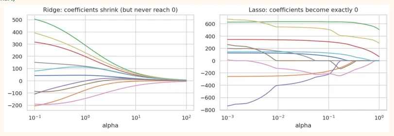
In the Lasso column many coefficients are exactly 0 : Lasso itself declared those features useless ( automatic feature selection ). In Ridge the coefficients became small but did not become 0.
The journey of the coefficients as alpha changes (coefficient path)
from sklearn.linear_model import lasso_path
alphas = np.logspace(-3, 0, 60)
ridge_coefs = np.array([Ridge(alpha=a * 100).fit(X_train, y_train).coef_ for a in alphas])
lasso_alphas, lasso_coefs, _ = lasso_path(X_train, y_train, alphas=alphas)
fig, axes = plt.subplots(1, 2, figsize=(11, 3.8)) axes[0].plot(alphas * 100, ridge_coefs) axes[0].set_xscale("log") axes[0].set_title("Ridge: coefficients shrink (but never reach 0)") axes[0].set_xlabel("alpha") axes[1].plot(lasso_alphas, lasso_coefs.T) axes[1].set_xscale("log") axes[1].set_title("Lasso: coefficients become exactly 0") axes[1].set_xlabel("alpha") plt.tight_layout() plt.show() OUTPUT (chart)
How to choose the best alpha? (Cross-Validation)
Alpha is a hyperparameter . To choose it, RidgeCV and LassoCV do cross-validation themselves and find the best alpha.
from sklearn.linear_model import RidgeCV, LassoCV
ridge_cv = make_pipeline(StandardScaler(), RidgeCV(alphas=np.logspace(-2, 3, 30),
cv=5)).fit(X_train, y_train)
lasso_cv = make_pipeline(StandardScaler(), LassoCV(cv=5, random_state=0)).fit(X_train,
y_train)
print("Ridge: best alpha =", round(ridge_cv[-1].alpha_, 2), "| test R2 =", round(ridge_cv.score(X_test, y_test), 3)) print("Lasso: best alpha =", round(lasso_cv[-1].alpha_, 3), "| test R2 =", round(lasso_cv.score(X_test, y_test), 3)) print("Features Lasso set to 0:", [c for c, v in zip(X.columns, lasso_cv[-1].coef_) if v == 0]) OUTPUT Ridge: best alpha = 41.75 | test R2 = 0.461 Lasso: best alpha = 1.655 | test R2 = 0.471 Features Lasso set to 0: ['age', 's2', 's4']
13.6 Hands-on
On the Diabetes dataset:
-
Baseline: find the test R² and RMSE of DummyRegressor (which predicts the average). How much better is linear regression than that?
-
Scaling + Ridge: find the test R² at alpha = 0.01, 1, 10, 100 and plot it.
-
Lasso: how many features become 0 at alpha = 0.5?
-
Gradient Descent: write the by-hand code above for multiple features (after applying StandardScaler to X_train).
-
Polynomial: using only the bmi feature of diabetes, build models from degree 1 to 8 and plot the train/test R².
from sklearn.dummy import DummyRegressor
base = DummyRegressor().fit(X_train, y_train) print("Baseline R2:", round(base.score(X_test, y_test), 3), "| RMSE:", round(np.sqrt(mean_squared_error(y_test, base.predict(X_test))), 2)) print("Linear R2:", round(lin.score(X_test, y_test), 3), "| RMSE:", round(np.sqrt(mean_squared_error(y_test, lin.predict(X_test))), 2)) OUTPUT Baseline R2: -0.012 | RMSE: 73.22 Linear R2: 0.453 | RMSE: 53.85 X_tr_s = StandardScaler().fit(X_train) for a in [0.01, 1, 10, 100]: r = Ridge(alpha=a).fit(X_tr_s.transform(X_train), y_train) print(f"alpha = {a:>6}: test R2 = {r.score(X_tr_s.transform(X_test), y_test):.3f}") OUTPUT alpha = 0.01: test R2 = 0.453 alpha = 1: test R2 = 0.454 alpha = 10: test R2 = 0.457 alpha = 100: test R2 = 0.461 KEY TAKEAWAYS
-
We measure the model's error with a cost function (MSE). Training means reducing the cost.
-
Gradient Descent: small steps (the learning rate) opposite to the slope. The foundation of every ML and deep learning model.
-
Learning rate too small = slow, too large = diverges. Always look at the cost graph.
-
Scale the features for gradient descent. Batch, Stochastic, Mini-batch: how much data at each step.
-
The Normal Equation gives the solution directly (on few features); gradient descent works on everything.
-
Polynomial regression learns a curve, but overfits when the degree grows (coefficients become very large).
-
• Ridge (L2): small coefficients. Lasso (L1): some exactly 0 (feature selection). ElasticNet: both. Choose alpha by cross-validation, scale first.