Chapter 14: Logistic Regression and Classification Metrics
MODULE 4 | WEEK 14
Chapter 14: Logistic Regression and Classification Metrics
So far we have predicted a number (regression). Now we will predict a category (classification): is an email spam or not, does a patient have the disease or not, will a customer leave the service or not. In this chapter we will learn Logistic Regression and the most important thing of all, evaluating a classification model the right way .
14.1 The classification problem
For example: looking at a student's study hours , predict whether they will pass (1) or fail (0). Let us apply linear regression and see what happens:
import numpy as np
import pandas as pd
import matplotlib.pyplot as plt
from sklearn.linear_model import LinearRegression, LogisticRegression
np.random.seed(3)
hours = np.sort(np.random.uniform(0, 10, 40))
passed = (hours + np.random.normal(0, 1.6, 40) > 5).astype(int)
H = hours.reshape(-1, 1)
xs = np.linspace(-1, 11, 200).reshape(-1, 1)
lin = LinearRegression().fit(H, passed)
log = LogisticRegression().fit(H, passed)
fig, axes = plt.subplots(1, 2, figsize=(11, 3.8))
axes[0].scatter(hours, passed, color="#6B5B95")
axes[0].plot(xs, lin.predict(xs), color="red")
axes[0].set_title("Linear Regression: goes below 0 and above 1")
axes[0].set_ylim(-0.5, 1.5)
axes[1].scatter(hours, passed, color="#6B5B95")
axes[1].plot(xs, log.predict_proba(xs)[:, 1], color="green")
axes[1].set_title("Logistic Regression: always between 0 and 1")
axes[1].set_ylim(-0.5, 1.5)
for ax in axes:
    ax.set_xlabel("Study hours")
    ax.set_ylabel("Pass (1) / Fail (0)")
plt.tight_layout()
plt.show()
OUTPUT (chart)
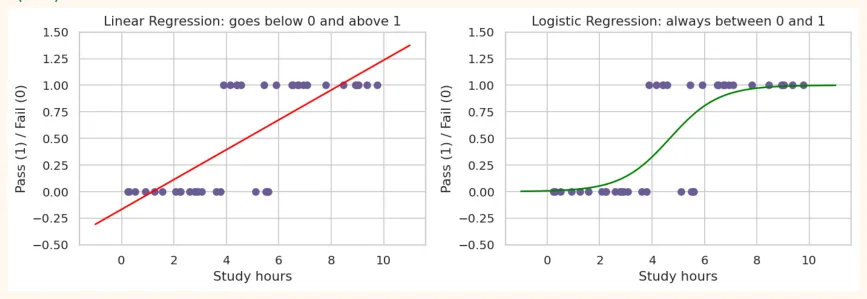
The straight line of linear regression gives meaningless values like -0.2 or 1.3 (a probability is never negative or above 1). We need a line that always stays between 0 and 1 and changes in an S-shape . That is the sigmoid .
14.2 Sigmoid and Logistic Regression
Sigmoid function: sigma(z) = 1 / (1 + e^(-z)) . It turns any number z into a value (probability) between 0 and 1 .
z = np.linspace(-8, 8, 200)
sigmoid = 1 / (1 + np.exp(-z))
plt.figure(figsize=(7, 3.6)) plt.plot(z, sigmoid, color="#A4457A", linewidth=2) plt.axhline(0.5, color="gray", linestyle="--") plt.axvline(0, color="gray", linestyle="--") plt.title("Sigmoid function: probability 0.5 at z = 0") plt.xlabel("z") plt.ylabel("sigmoid(z)") plt.show() OUTPUT (chart)
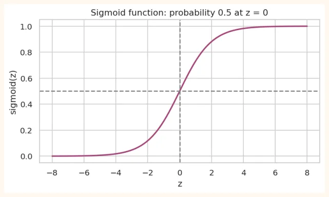
The way Logistic Regression works:
-
First compute a score like linear regression: z = b0 + b1 x1 + b2 x2 + ...
-
Pass z through the sigmoid: probability = sigmoid(z) (from 0 to 1).
-
Decision: if probability >= 0.5 (the threshold) then class 1, otherwise class 0.
The loss of Logistic Regression (Log Loss)
Linear regression had MSE. Logistic regression has Log Loss (Binary Cross-Entropy) : if the model predicts the correct class with confidence , the penalty is small, and if it predicts the wrong class with confidence , the penalty is very big. Training is then done with gradient descent (Chapter 13).
14.3 Logistic Regression in scikit-learn
Breast cancer dataset (569 patients, 30 measurements, 0 = malignant (harmful) , 1 = benign (not harmful) ):
from sklearn.datasets import load_breast_cancer from sklearn.model_selection import train_test_split from sklearn.preprocessing import StandardScaler from sklearn.pipeline import make_pipeline bc = load_breast_cancer(as_frame=True) X, y = bc.data, bc.target X_train, X_test, y_train, y_test = train_test_split(X, y, test_size=0.2, random_state=42, stratify=y) clf = make_pipeline(StandardScaler(), LogisticRegression(max_iter=1000)) clf.fit(X_train, y_train) print("Accuracy:", round(clf.score(X_test, y_test), 3)) print("First 5 predictions :", clf.predict(X_test)[:5]) print("First 5 probabilities(1):", clf.predict_proba(X_test)[:5, 1].round(3)) OUTPUT Accuracy: 0.982 First 5 predictions : [0 1 0 1 0] First 5 probabilities(1): [0. 1. 0.006 0.534 0. ]
predict() gives the class (0/1), while predict_proba() gives the probability of each class. The probability is always more valuable because with it you can choose the threshold yourself .
What the coefficients mean (odds)
The coefficients of logistic regression act on the log-odds . An easy way: compute exp(coefficient) , which is the odds ratio : how many times the odds of class 1 are multiplied when the feature increases by 1 (scaled) unit.
coefs = pd.Series(clf[-1].coef_[0], index=X.columns) top = coefs.reindex(coefs.abs().sort_values(ascending=False).index)[:6] print(top.round(2)) print("\nOdds ratio (exp(coef)) of the first feature:", round(np.exp(top.iloc[0]), 3)) OUTPUT worst texture -1.26 radius error -1.08 worst concave points -0.95 worst area -0.95 worst radius -0.95 worst symmetry -0.94 dtype: float64
Odds ratio (exp(coef)) of the first feature: 0.285
For example the odds ratio of worst texture is 0.285: when this feature increases by 1 std , the odds of being benign become about 71% lower . A feature with a negative coefficient pushes toward malignant (0) , and one
with a positive coefficient toward benign (1). This is why logistic regression is considered an easy-to-understand (interpretable) model, which matters a lot in fields like medicine and banking.
Decision Boundary
On two features, logistic regression separates class 0 and class 1 with a straight line :
from sklearn.datasets import make_classification
from sklearn.inspection import DecisionBoundaryDisplay
Xd, yd = make_classification(n_samples=200, n_features=2, n_redundant=0, n_informative=2,
                             n_clusters_per_class=1, class_sep=1.2, random_state=4)
lr2 = LogisticRegression().fit(Xd, yd)
fig, ax = plt.subplots(figsize=(6, 4.2))
DecisionBoundaryDisplay.from_estimator(lr2, Xd, response_method="predict_proba",
cmap="RdBu_r",
alpha=0.5, ax=ax, plot_method="pcolormesh",
shading="auto")
ax.scatter(Xd[:, 0], Xd[:, 1], c=yd, cmap="coolwarm", edgecolor="white")
ax.set_title("Decision boundary of Logistic Regression (straight line)")
plt.show()
OUTPUT (chart)
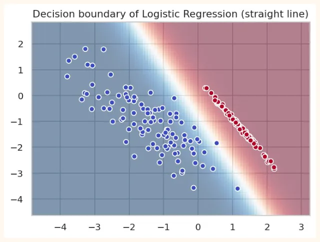
Deep red or blue area = the model is very sure about the class, the white area in the middle = 50-50 (the boundary). Notice: logistic regression can only make a straight (linear) boundary. For complex shapes, other algorithms will come.
14.4 Multiclass Classification
For more than two classes (like the 3 species of Iris), logistic regression uses softmax : it computes the probability of every class, and they all add up to 1.
from sklearn.datasets import load_iris
iris = load_iris(as_frame=True)
Xi_train, Xi_test, yi_train, yi_test = train_test_split(iris.data, iris.target,
test_size=0.2,
random_state=42,
stratify=iris.target)
multi = make_pipeline(StandardScaler(), LogisticRegression(max_iter=1000)).fit(Xi_train,
yi_train)
print("Accuracy:", round(multi.score(Xi_test, yi_test), 3)) print("Probabilities for one flower (setosa, versicolor, virginica):") print(multi.predict_proba(Xi_test.iloc[[0]]).round(3), "-> sum of all =", multi.predict_proba(Xi_test.iloc[[0]]).sum()) OUTPUT Accuracy: 0.933 Probabilities for one flower (setosa, versicolor, virginica): [[0.979 0.021 0. ]] -> sum of all = 1.0
Regularization: the parameter C
The regularization parameter in logistic regression is C , and it is the opposite of alpha : small C = more penalty (simple model) , large C = less penalty . The default is C = 1.
for C in [0.001, 0.01, 1, 100]: m = make_pipeline(StandardScaler(), LogisticRegression(C=C, max_iter=2000)).fit(X_train, y_train) print(f"C = {C:>6}: train = {m.score(X_train, y_train):.3f} | test = {m.score(X_test, y_test):.3f}") OUTPUT C = 0.001: train = 0.888 | test = 0.930 C = 0.01: train = 0.956 | test = 0.947 C = 1: train = 0.989 | test = 0.982 C = 100: train = 0.993 | test = 0.947
14.5 Evaluating Classification: the Confusion Matrix
Accuracy alone is not enough. We also need to know what kind of mistakes the model is making. For this we have the Confusion Matrix . Example of cancer detection ( Positive = has the disease ):
| Model said: NOT sick | Model said: SICK | |
|---|---|---|
| Actually NOT sick | TN(True Negative): correct, called a healthy person healthy | FP(False Positive): wrong, called a healthy person sick (false alarm) |
| Actually SICK | FN(False Negative): wrong, called a sick person healthy (dangerous!) | TP(True Positive): correct, called a sick person sick |
14.6 Accuracy, Precision, Recall, F1
| Metric | Formula | The question it answers |
|---|---|---|
| Accuracy | (TP + TN) / total | How many of all the predictions were correct? |
| Precision | TP / (TP + FP) | When the model said "positive", how often was it right? (how many false alarms?) |
| Recall(Sensitivity) | TP / (TP + FN) | Of all the actual positives, how many did we catch? (how many were missed?) |
| Specificity | TN / (TN + FP) | Of all the actual negatives, how many were identified correctly? |
| F1-score | 2 x P x R / (P + R) | A balanced combination of Precision and Recall |
Which metric when?
| Situation | What matters more | Example |
|---|---|---|
| FN is very costly | Recall | Cancer detection, catching fraud, fire alarm |
| FP is very costly | Precision | Spam filter (calling an important email spam), accusing an innocent person of a crime |
| Balance of both needed | F1-score | General classification, imbalanced data |
| Classes are balanced | Accuracy is also fine | A dataset with balanced classes |
14.7 Imbalanced Data and the Deception of Accuracy
In fraud detection only 10 out of 1000 transactions are fraud (1%). A model that always says "not fraud" will have 99% accuracy, but it does not catch a single fraud . This is the Accuracy Paradox .
np.random.seed(0) y_true = np.array([1] * 10 + [0] * 990) # 1% fraud y_lazy = np.zeros(1000, dtype=int) # always "not fraud" print("Accuracy:", accuracy_score(y_true, y_lazy)) print("Recall :", recall_score(y_true, y_lazy)) # 0.0: caught none OUTPUT Accuracy: 0.99 Recall : 0.0
For imbalanced data look at precision, recall, F1, ROC-AUC , and try these approaches:
-
class_weight="balanced" (more weight to the small class): LogisticRegression(class_weight="balanced") .
-
Oversampling / Undersampling (increasing the points of the small class or reducing those of the big class). SMOTE is a well-known method.
-
Changing the threshold (see below).
-
Split with stratify=y , and stratified cross-validation.
14.8 ROC Curve and AUC
Logistic regression gives a probability, and the threshold (default 0.5) decides the class. Changing the threshold changes precision and recall. The ROC curve shows the model's performance at every possible threshold in a single chart:
-
Y-axis: TPR (True Positive Rate = Recall).
-
X-axis: FPR (False Positive Rate = FP / (FP + TN)): the false alarms.
-
The curve of a best model goes toward the top-left corner. The straight diagonal line = a blind guess (random).
-
AUC (Area Under Curve): the area under the curve. 1.0 = perfect , 0.5 = random .
from sklearn.metrics import roc_curve, roc_auc_score
from sklearn.ensemble import RandomForestClassifier
proba = clf.predict_proba(X_test)[:, 1]
rf = RandomForestClassifier(random_state=0).fit(X_train, y_train)
proba_rf = rf.predict_proba(X_test)[:, 1]
plt.figure(figsize=(5.6, 4.6)) for name, p, color in [("Logistic Regression", proba, "#A4457A"), ("Random Forest", proba_rf, "#2F7D4F")]: fpr, tpr, _ = roc_curve(y_test, p) plt.plot(fpr, tpr, color=color, linewidth=2, label=f"{name} (AUC = {roc_auc_score(y_test, p):.3f})") plt.plot([0, 1], [0, 1], linestyle="--", color="gray", label="Random guess (AUC = 0.5)") plt.xlabel("False Positive Rate (false alarms)") plt.ylabel("True Positive Rate (Recall)") plt.title("ROC curve") plt.legend(loc="lower right") plt.show() OUTPUT (chart)
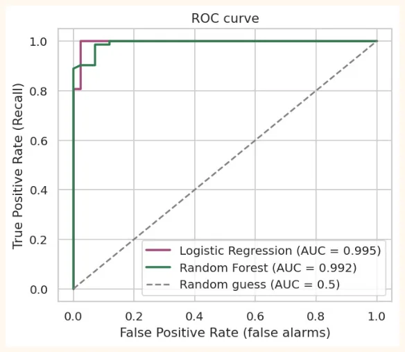
Threshold tuning: increasing recall
If recall matters in cancer detection (sick people should not be missed), we can lower the threshold. Then the model puts more people under "suspicion": recall rises but precision falls.
p_malignant = clf.predict_proba(X_test)[:, 0]          # probability of malignant (class 0)
actual_malignant = (y_test == 0).values
for thr in [0.5, 0.2, 0.05, 0.01]:
    flagged = p_malignant >= thr                       # called these "malignant"
    tp = (flagged & actual_malignant).sum()
fp = (flagged & ~actual_malignant).sum() fn = (~flagged & actual_malignant).sum() print(f"threshold {thr}: caught = {tp}, false alarms = {fp}, missed = {fn}") OUTPUT
threshold 0.5: caught = 41, false alarms = 1, missed = 1
threshold 0.2: caught = 41, false alarms = 6, missed = 1
threshold 0.05: caught = 42, false alarms = 18, missed = 0 threshold 0.01: caught = 42, false alarms = 30, missed = 0 At threshold 0.5 one malignant case was missed (FN = 1). When the threshold was lowered to 0.05 it was caught too (FN = 0), but false alarms (FP) rose from 1 to 18 : 18 healthy people were also put under "suspicion". This is the trade-off between precision and recall . Which threshold to choose depends on the business/medical need (in cancer perhaps recall matters more, in a spam filter precision), not just on the data.
14.9 Hands-on
-
Baseline: on breast cancer, find the accuracy and recall (for malignant) of DummyClassifier(strategy="most_frequent").
-
Effect of C: compare the test accuracy and ROC-AUC at C = 0.01, 0.1, 1, 10.
-
class_weight: apply LogisticRegression(class_weight="balanced") and look at the confusion matrix. Did recall improve?
-
Threshold: in the code of 14.8 also try thresholds 0.05 and 0.9. When does FN become 0, and what is the cost of that?
-
Thinking question: which metric will matter more for a spam filter, and why? (Which is costly, FP or FN?)
from sklearn.dummy import DummyClassifier
dummy = DummyClassifier(strategy="most_frequent").fit(X_train, y_train)
print("Baseline accuracy:", round(dummy.score(X_test, y_test), 3))
print("Baseline recall (malignant):", recall_score(y_test, dummy.predict(X_test),
pos_label=0))
balanced = make_pipeline(StandardScaler(), LogisticRegression(class_weight="balanced",
max_iter=1000)).fit(X_train, y_train)
print("Balanced model recall (malignant):", round(recall_score(y_test,
balanced.predict(X_test), pos_label=0), 3))
print("Normal model recall (malignant)  :", round(recall_score(y_test, pred, pos_label=0),
3))
OUTPUT
Baseline accuracy: 0.632
Baseline recall (malignant): 0.0
Balanced model recall (malignant): 0.976
Normal model recall (malignant)  : 0.976
KEY TAKEAWAYS
-
In classification we predict a category. Logistic Regression is a classification algorithm (despite having regression in its name).
-
The sigmoid turns a score into a probability from 0 to 1. The class is decided by the threshold (default 0.5).
-
predict() gives the class, predict_proba() gives the probability. From the coefficients we get the odds ratio (an interpretable model).
-
C is the regularization parameter (the opposite of alpha): small C = more penalty.
-
Confusion Matrix: TP, FP, FN, TN. FP = false alarm, FN = missed (often more dangerous).
-
Precision = of those called positive, the correct ones. Recall = of the actual positives, those caught. F1 is the balance of both.
-
On imbalanced data accuracy deceives. ROC-AUC is independent of the threshold (1 is best, 0.5 is random). Choose the threshold from the business need.