Chapter 13: Linear Regression Deep Dive, Gradient Descent aur Regularization
MODULE 4 | WEEK 13
Chapter 13: Linear Regression Deep Dive, Gradient Descent aur Regularization
Module 3 me hum ne linear regression statistics ke nazariye se dekhi. Ab hum usay ML ke nazariye se dekhte hain: model seekhta kaise hai ? Is ka jawab hai Gradient Descent , wohi idea jo neural networks ke training me bhi chalta hai. Phir Regularization (L1, L2) seekhenge, jo model ko overfitting se bachati hai.
13.1 Cost Function: model ki galti ka paimana
Linear regression ki lakeer y = w x + b hai (yahan w slope aur b intercept). Hamein w aur b ki wo values chahiye jin par model ki galti sab se kam ho. Galti napne ke liye hum cost function (ya loss function) banate hain. Linear regression me aam taur par MSE (Mean Squared Error) hota hai:
J(w, b) = (1/n) x sum( (andaza - asli)<sup>2</sup> )
OUTPUT (chart)
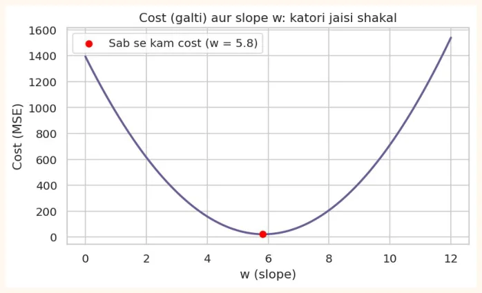
13.2 Gradient Descent
Gradient ka matlab hai dhalan (slope of the cost) : ye batata hai ke parameter ko barhane se cost barhega ya ghatega. Hum parameter ko dhalan ke ulte rukh thora sa badalte hain.
w = w - alpha x (dJ/dw) aur b = b - alpha x (dJ/db)
-
alpha (learning rate): qadam ka size. Bohat chhota to dheere pohanchoge, bohat bara to wadi ke upar se uchhal jaoge.
-
dJ/dw: w badalne par cost kitna badalta hai (derivative / dhalan).
-
Ye amal bar bar (iterations) dohraya jata hai jab tak cost ghatna band na ho jaye.
MSE ke liye derivatives ye hain (n = samples ki tadaad, error = andaza - asli):
-
dJ/dw = (2/n) x sum(error x x)
-
dJ/db = (2/n) x sum(error)
Hath se (NumPy me) Gradient Descent
Pehle x ko scale karte hain (wajah neeche samjhayenge), phir loop chalate hain:
x = (hours - hours.mean()) / hours.std()       # scaled feature
y = marks
w, b = 0.0, 0.0           # shuru me dono 0
lr = 0.1                  # learning rate
n = len(x)
history = []
for i in range(100):
    pred = w * x + b
    error = pred - y
    history.append((error ** 2).mean())        # cost note karo
    dw = (2 / n) * (error * x).sum()
    db = (2 / n) * error.sum()
    w = w - lr * dw
    b = b - lr * db
    if i in (0, 1, 5, 20, 99):
        print(f"iteration {i + 1:>3}: w = {w:6.2f}, b = {b:6.2f}, cost = {history[-
1]:8.2f}")
OUTPUT
iteration   1: w =   2.86, b =  13.84, cost =  5012.34
iteration   2: w =   5.14, b =  24.91, cost =  3215.60
iteration   6: w =  10.54, b =  51.05, cost =   557.29
iteration  21: w =  14.15, b =  68.55, cost =    22.05
iteration 100: w =  14.28, b =  69.19, cost =    21.39
Cost har iteration par ghat raha hai aur w, b settle ho rahe hain. Ab ye parameters wapas original scale me la kar polyfit (sahi jawab) se milate hain:
slope = w / hours.std()
intercept = b - slope * hours.mean()
print("Gradient Descent:", round(slope, 3), round(intercept, 3))
b1, b0 = np.polyfit(hours, marks, 1)
print("polyfit (sahi)  :", round(b1, 3), round(b0, 3))
OUTPUT
Gradient Descent: 5.829 35.135
polyfit (sahi)  : 5.829 35.135
fig, axes = plt.subplots(1, 2, figsize=(11, 3.6))
axes[0].plot(history, color="#A4457A", linewidth=2)
axes[0].set_title("Cost har iteration par kam hota hua")
axes[0].set_xlabel("Iteration")
axes[0].set_ylabel("Cost (MSE)")
axes[1].scatter(hours, marks, color="#6B5B95", s=18)
xs = np.linspace(1, 10, 50)
axes[1].plot(xs, intercept + slope * xs, color="red", linewidth=2)
axes[1].set_title("Gradient Descent ki seekhi hui lakeer")
axes[1].set_xlabel("Ghantay")
axes[1].set_ylabel("Marks")
plt.tight_layout()
plt.show()
OUTPUT (chart)
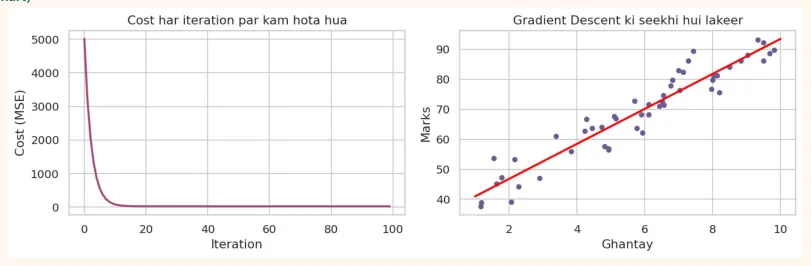
Learning rate ka asar
def gradient_descent(x, y, lr, iters=60):
    w = b = 0.0
    n = len(x)
    costs = []
    for _ in range(iters):
error = w * x + b - y costs.append((error ** 2).mean()) w -= lr * (2 / n) * (error * x).sum() b -= lr * (2 / n) * error.sum() return costs for lr in [0.001, 0.3, 1.05]: c = gradient_descent(x, y, lr) print(f"lr = {lr:>5}: shuru ka cost = {c[0]:8.1f} | aakhri cost = {c[-1]:.3g}") OUTPUT
lr = 0.001: shuru ka cost =   5012.3 | aakhri cost = 3.96e+03
lr =   0.3: shuru ka cost =   5012.3 | aakhri cost = 21.4
lr =  1.05: shuru ka cost =   5012.3 | aakhri cost = 3.82e+08
fig, axes = plt.subplots(1, 3, figsize=(13, 3.4))
for ax, lr, title in zip(axes, [0.001, 0.3, 1.05],
                         ["Bohat chhota (lr = 0.001)\nbohat dheere", "Munasib (lr = 0.3)\
nsahi", "Bohat bara (lr = 1.05)\ncost barhta gaya"]):
    ax.plot(gradient_descent(x, y, lr, iters=30), color="#6B5B95", linewidth=2)
    ax.set_title(title)
    ax.set_xlabel("Iteration")
axes[0].set_ylabel("Cost")
axes[2].set_yscale("log")
plt.tight_layout()
plt.show()
OUTPUT (chart)
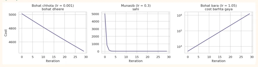
PRACTICAL TIP
Learning rate sab se ahem hyperparameters me se ek hai. Aam shuruaat: 0.1, 0.01, 0.001 aazma kar cost ka graph dekhna. Agar cost barh raha ho to learning rate kam karo.
Feature Scaling gradient descent ke liye kyun zaroori hai?
Agar features ka scale bohat alag ho (ek 0 se 1, doosra 0 se 100,000) to cost ki "katori" ek lambi tang nali ban jati hai, aur gradient descent us me zig-zag karta hai aur bohat dheere pohanchta hai (ya diverge karta hai). Scaling se katori gol ho jati hai aur seedha neeche pohanchta hai.
# Same learning rate (0.01), same iterations, magar scaled vs unscaled x
print("Scaled x   :", round(gradient_descent(x, y, 0.01, iters=200)[-1], 2))
print("Unscaled x :", round(gradient_descent(hours, y, 0.01, iters=200)[-1], 2))
print("Sab se kam mumkin cost:", round(((np.polyval(np.polyfit(hours, marks, 1), hours) -
marks) ** 2).mean(), 2))
OUTPUT
Scaled x   : 23.0
Unscaled x : 73.82
Sab se kam mumkin cost: 21.39
Scaled data wala cost sab se kam mumkin cost ke qareeb pohanch gaya, jab ke unscaled wala abhi door hai.
Gradient Descent ki qismein
| Qism | Kitna data har qadam par | Khasusiyat |
|---|---|---|
| Batch | Pooratraining data | Sahi aur stable, magar bare data par slow |
| Stochastic (SGD) | Eksample | Tez, shor wala (lakeer idhar udhar hoti hai), bare data ke liye acha |
| Mini-batch | Chhote batches (jaise 32 ya 64 samples) | Dono ka sunehra darmiyan,deep learning me sab se aam |
from sklearn.linear_model import SGDRegressor
sgd = SGDRegressor(max_iter=2000, tol=1e-4, random_state=0)
sgd.fit(x.reshape(-1, 1), y)
print("SGD slope, intercept (scaled x par):", round(sgd.coef_[0], 2),
round(sgd.intercept_[0], 2))
print("Hamare hath wale:                   ", round(w, 2), round(b, 2))
OUTPUT
SGD slope, intercept (scaled x par): 14.28 69.17
Hamare hath wale:                    14.28 69.19
Normal Equation: gradient descent ke baghair seedha hal
Linear regression ka ek formula bhi hai jo seedha best w deta hai: w = (X<sup>T</sup> X)<sup>-1</sup> X<sup>T</sup> y . Scikit-learn ka LinearRegression aam taur par isi (ya isi jaisi cheez) se kaam leta hai.
| Normal Equation | Gradient Descent | |
|---|---|---|
| Learning rate | Zaroorat nahi | Chunna parta hai |
| Iterations | Koi nahi, ek bar me | Bohat |
| Features zyada (lakhon) | Slow(matrix inverse mehnga) | Tez |
| Samples bohat zyada | Slow ho sakta hai | Mini-batch se aasani |
| Kis par kaam | Sirf linear regression | Harcheez par (logistic, neural networks...) |
Isi liye gradient descent itna ahem hai: wo sirf linear regression nahi, har ML aur deep learning model ko train karne ka bunyadi tareeqa hai.
13.3 Multiple Linear Regression (scikit-learn ke saath)
Ab ek asli dataset: Diabetes (442 mareez, 10 napayiyan jaise umar, BMI, blood pressure, aur target: ek saal baad bimari ki pesh-raft ka paimana). Is data ke features pehle se scale kiye hue hain.
from sklearn.datasets import load_diabetes
from sklearn.model_selection import train_test_split
from sklearn.linear_model import LinearRegression
from sklearn.metrics import mean_squared_error, r2_score
data = load_diabetes(as_frame=True)
X, y = data.data, data.target
print(X.shape)
print(X.columns.tolist())
X_train, X_test, y_train, y_test = train_test_split(X, y, test_size=0.2, random_state=42)
lin = LinearRegression().fit(X_train, y_train)
pred = lin.predict(X_test)
print("Test R2  :", round(r2_score(y_test, pred), 3))
print("Test RMSE:", round(np.sqrt(mean_squared_error(y_test, pred)), 2))
print(pd.Series(lin.coef_, index=X.columns).round(1))
OUTPUT
(442, 10)
['age', 'sex', 'bmi', 'bp', 's1', 's2', 's3', 's4', 's5', 's6']
Test R2  : 0.453
Test RMSE: 53.85
age     37.9
sex   -242.0
bmi    542.4
bp     347.7
s1    -931.5
s2     518.1
s3     163.4
s4     275.3
s5     736.2
s6      48.7
dtype: float64
Dhyan do: kuch coefficients bohat bare hain (jaise s1 aur s2 ke), jo shak paida karta hai ke ye features aapas me bohat judte hain. Jab aisa ho to model bohat sensitive ho jata hai, aur yahin regularization madad karti hai.
13.4 Polynomial Regression aur Overfitting
Agar rishta seedhi lakeer ka na ho, to hum features ke powers (x<sup>2</sup> , x<sup>3</sup> ...) jor kar model ko curve seekhne ke qabil bana sakte hain. Isay Polynomial Regression kehte hain. Wo ab bhi linear regression hi hai (coefficients me linear), bas features badal gaye.
from sklearn.preprocessing import PolynomialFeatures, StandardScaler
from sklearn.pipeline import make_pipeline
PolynomialFeatures(degree=3, include_bias=False).fit_transform(np.array([[2.0]]))   # 2 ->
[2, 4, 8]
Magar degree barhane ka matlab hai zyada pecheeda model , aur kam data par overfitting ka khatra:
np.random.seed(4)
xp = np.sort(np.random.uniform(0, 1, 25))
yp = np.sin(2 * np.pi * xp) + np.random.normal(0, 0.25, 25)
xs = np.linspace(0, 1, 200).reshape(-1, 1)
m_over = make_pipeline(PolynomialFeatures(12), StandardScaler(),
LinearRegression()).fit(xp.reshape(-1, 1), yp)
coefs = m_over.named_steps["linearregression"].coef_
print("Degree 12 ke sab se bare 3 coefficients (absolute):", np.sort(np.abs(coefs))[-
3:].round(0))
OUTPUT
Degree 12 ke sab se bare 3 coefficients (absolute): [17897428. 25923396. 26330352.]
Coefficients lakhon aur karoron me hain! Jab model overfit hota hai to wo data ko chhoone ke liye bohat bare bare coefficients istemal karta hai jo ek doosre ko cancel karte hain. Ye hi regularization ka sab se ahem insight hai.
13.5 Regularization: model ko "sakht" banana
Regularization ka idea: cost function me ek saza (penalty) jorna jo bare coefficients ko pasand na kare, taake model saada rahe aur data ko ratta na lagaye.
Naya cost = MSE + penalty
OUTPUT (chart)
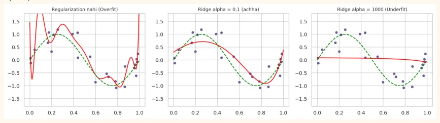
Same degree-12 model hai, magar Ridge ki saza ne lakeer ko smooth kar diya. Alpha bohat bara karne par model ab itna saada ho gaya ke lagbhag seedhi lakeer ban gayi (underfit).
Ridge, Lasso aur ElasticNet asli data par
from sklearn.linear_model import Ridge, Lasso, ElasticNet
models = {
    "Linear": LinearRegression(),
    "Ridge (alpha=0.1)": Ridge(alpha=0.1),
    "Lasso (alpha=0.1)": Lasso(alpha=0.1),
    "ElasticNet": ElasticNet(alpha=0.001, l1_ratio=0.5),
}
rows = {}
for name, m in models.items():
    m.fit(X_train, y_train)
    rows[name] = m.coef_.round(1)
    print(f"{name:19s} test R2 = {m.score(X_test, y_test):.3f}")
print(pd.DataFrame(rows, index=X.columns))
OUTPUT
Linear              test R2 = 0.453
Ridge (alpha=0.1)   test R2 = 0.461
Lasso (alpha=0.1)   test R2 = 0.472
ElasticNet          test R2 = 0.461
     Linear  Ridge (alpha=0.1)  Lasso (alpha=0.1)  ElasticNet
age    37.9               42.9                0.0        43.4
sex  -242.0             -205.5             -152.7      -183.7
bmi   542.4              505.1              552.7       472.6
bp    347.7              317.1              303.4       300.3
s1   -931.5             -108.5              -81.4       -74.5
s2    518.1              -86.2               -0.0       -88.6
s3    163.4             -190.4             -229.3      -192.8
s4    275.3              151.7                0.0       144.2
s5    736.2              392.3              447.9       361.1
s6     48.7               79.9               29.6        92.0
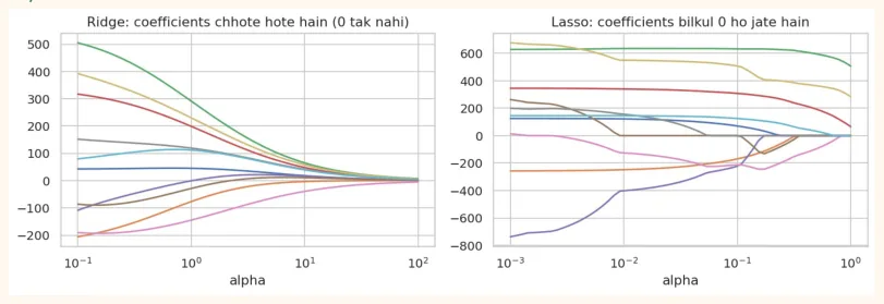
Lasso wale column me kai coefficients bilkul 0 hain: Lasso ne un features ko khud hi bekar qarar de diya ( automatic feature selection ). Ridge me coefficients chhote ho gaye magar 0 nahi hue.
Alpha badalne par coefficients ka safar (coefficient path)
from sklearn.linear_model import lasso_path
alphas = np.logspace(-3, 0, 60)
ridge_coefs = np.array([Ridge(alpha=a * 100).fit(X_train, y_train).coef_ for a in alphas])
lasso_alphas, lasso_coefs, _ = lasso_path(X_train, y_train, alphas=alphas)
fig, axes = plt.subplots(1, 2, figsize=(11, 3.8))
axes[0].plot(alphas * 100, ridge_coefs)
axes[0].set_xscale("log")
axes[0].set_title("Ridge: coefficients chhote hote hain (0 tak nahi)")
axes[0].set_xlabel("alpha")
axes[1].plot(lasso_alphas, lasso_coefs.T)
axes[1].set_xscale("log")
axes[1].set_title("Lasso: coefficients bilkul 0 ho jate hain")
axes[1].set_xlabel("alpha")
plt.tight_layout()
plt.show()
OUTPUT (chart)
Behtareen alpha kaise chunein? (Cross-Validation)
Alpha ek hyperparameter hai. Isay chunne ke liye RidgeCV aur LassoCV khud cross-validation karke behtareen alpha dhoond dete hain.
from sklearn.linear_model import RidgeCV, LassoCV
ridge_cv = make_pipeline(StandardScaler(), RidgeCV(alphas=np.logspace(-2, 3, 30),
cv=5)).fit(X_train, y_train)
lasso_cv = make_pipeline(StandardScaler(), LassoCV(cv=5, random_state=0)).fit(X_train,
y_train)
print("Ridge: behtareen alpha =", round(ridge_cv[-1].alpha_, 2), "| test R2 =",
round(ridge_cv.score(X_test, y_test), 3))
print("Lasso: behtareen alpha =", round(lasso_cv[-1].alpha_, 3), "| test R2 =",
round(lasso_cv.score(X_test, y_test), 3))
print("Lasso ne 0 kiye hue features:", [c for c, v in zip(X.columns, lasso_cv[-1].coef_) if
v == 0])
OUTPUT
Ridge: behtareen alpha = 41.75 | test R2 = 0.461
Lasso: behtareen alpha = 1.655 | test R2 = 0.471
Lasso ne 0 kiye hue features: ['age', 's2', 's4']
AAM GALTIYAN
-
Regularization se pehle scaling na karna.
-
alpha ko randomly chun lena. Cross-validation (RidgeCV/LassoCV) use karo.
-
Gradient descent me learning rate par dhyan na dena aur cost ka graph na dekhna.
-
Samajhna ke regularization hamesha test score behtar karti hai. Jab model pehle se saada ho to ye nuqsan bhi kar sakti hai.
-
Intercept ko regularize karna. Scikit-learn me wo khud alag rakha jata hai.
-
Lasso me bohat zyada correlated features ho to wo unme se kisi ek ko random chun leta hai. Aise me ElasticNet behtar hai.
13.6 Hands-on
Diabetes dataset par:
-
Baseline: DummyRegressor (average batane wala) ka test R<sup>2</sup> aur RMSE nikalo. Linear regression usse kitna behtar hai?
-
Scaling + Ridge: alpha = 0.01, 1, 10, 100 par test R<sup>2</sup> nikalo aur plot karo.
-
Lasso: alpha = 0.5 par kitne features 0 ho jate hain?
-
Gradient Descent: upar wale hath ke code ko multiple features (X_train ko StandardScaler karke) ke liye likho.
-
Polynomial: diabetes ke sirf bmi feature se degree 1 se 8 tak models banao aur train/test R<sup>2</sup> plot karo.
from sklearn.dummy import DummyRegressor
base = DummyRegressor().fit(X_train, y_train)
print("Baseline R2:", round(base.score(X_test, y_test), 3), "| RMSE:",
round(np.sqrt(mean_squared_error(y_test, base.predict(X_test))), 2))
print("Linear   R2:", round(lin.score(X_test, y_test), 3), "| RMSE:",
round(np.sqrt(mean_squared_error(y_test, lin.predict(X_test))), 2))
OUTPUT
Baseline R2: -0.012 | RMSE: 73.22
Linear   R2: 0.453 | RMSE: 53.85
X_tr_s = StandardScaler().fit(X_train)
for a in [0.01, 1, 10, 100]:
    r = Ridge(alpha=a).fit(X_tr_s.transform(X_train), y_train)
    print(f"alpha = {a:>6}: test R2 = {r.score(X_tr_s.transform(X_test), y_test):.3f}")
OUTPUT
alpha =   0.01: test R2 = 0.453
alpha =      1: test R2 = 0.454
alpha =     10: test R2 = 0.457
alpha =    100: test R2 = 0.461
KEY TAKEAWAYS
-
Model ki galti ko cost function (MSE) se napte hain. Training ka matlab cost ko kam karna hai.
-
Gradient Descent: dhalan ke ulte rukh chhote qadam (learning rate). Har ML aur deep learning model ki bunyad.
-
Learning rate bohat chhota = dheera, bohat bara = diverge. Cost ka graph zaroor dekho.
-
Gradient descent ke liye features scale karo. Batch, Stochastic, Mini-batch: kitna data har qadam par.
-
Normal Equation seedha hal deta hai (kam features par), gradient descent har cheez par chalta hai.
-
Polynomial regression curve seekhti hai, magar degree barhane par overfit ho jati hai (coefficients bohat bare).
-
Ridge (L2): coefficients chhote. Lasso (L1): kuch bilkul 0 (feature selection). ElasticNet: dono. alpha crossvalidation se chuno, scaling pehle karo.