Chapter 14: Logistic Regression aur Classification Metrics
MODULE 4 | WEEK 14
Chapter 14: Logistic Regression aur Classification Metrics
Ab tak hum ne number ka andaza lagaya (regression). Ab category ka andaza lagayenge (classification): email spam hai ya nahi, mareez ko bimari hai ya nahi, customer service chhor dega ya nahi. Is chapter me Logistic Regression aur sab se ahem cheez, classification model ko sahi tareeqe se parakhna , seekhenge.
14.1 Classification ka masla
Maslan: ek student ke parhai ke ghantay dekh kar andaza lagana ke wo pass (1) hoga ya fail (0). Hum linear regression laga kar dekhte hain to kya hota hai:
import numpy as np
import pandas as pd
import matplotlib.pyplot as plt
from sklearn.linear_model import LinearRegression, LogisticRegression
np.random.seed(3)
hours = np.sort(np.random.uniform(0, 10, 40))
passed = (hours + np.random.normal(0, 1.6, 40) > 5).astype(int)
H = hours.reshape(-1, 1)
xs = np.linspace(-1, 11, 200).reshape(-1, 1)
lin = LinearRegression().fit(H, passed)
log = LogisticRegression().fit(H, passed)
fig, axes = plt.subplots(1, 2, figsize=(11, 3.8))
axes[0].scatter(hours, passed, color="#6B5B95")
axes[0].plot(xs, lin.predict(xs), color="red")
axes[0].set_title("Linear Regression: 0 se neeche aur 1 se upar chali jati hai")
axes[0].set_ylim(-0.5, 1.5)
axes[1].scatter(hours, passed, color="#6B5B95")
axes[1].plot(xs, log.predict_proba(xs)[:, 1], color="green")
axes[1].set_title("Logistic Regression: hamesha 0 se 1 ke beech")
axes[1].set_ylim(-0.5, 1.5)
for ax in axes:
    ax.set_xlabel("Parhai ke ghantay")
    ax.set_ylabel("Pass (1) / Fail (0)")
plt.tight_layout()
plt.show()
OUTPUT (chart)
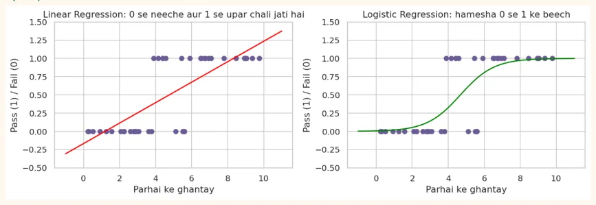
Linear regression ki seedhi lakeer -0.2 ya 1.3 jaisi be-maani values deti hai (probability kabhi manfi ya 1 se zyada nahi hoti). Hamein aisi lakeer chahiye jo hamesha 0 se 1 ke beech rahe aur ek S-shape bana kar badle. Ye sigmoid hai.
14.2 Sigmoid aur Logistic Regression
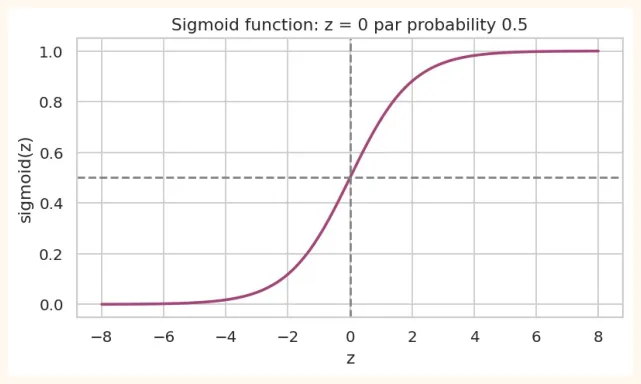
Sigmoid function: sigma(z) = 1 / (1 + e<sup>-z</sup> ) . Ye kisi bhi number z ko 0 se 1 ke beech ki value (probability) bana deta hai.
z = np.linspace(-8, 8, 200)
sigmoid = 1 / (1 + np.exp(-z))
plt.figure(figsize=(7, 3.6))
plt.plot(z, sigmoid, color="#A4457A", linewidth=2)
plt.axhline(0.5, color="gray", linestyle="--")
plt.axvline(0, color="gray", linestyle="--")
plt.title("Sigmoid function: z = 0 par probability 0.5")
plt.xlabel("z")
plt.ylabel("sigmoid(z)")
plt.show()
OUTPUT (chart)
Logistic Regression ka tareeqa:
-
Pehle linear regression jaisa score nikalo: z = b0 + b1 x1 + b2 x2 + ...
-
z ko sigmoid se guzaro: probability = sigmoid(z) (0 se 1).
-
Faisla: agar probability >= 0.5 (threshold) to class 1, warna class 0.
Logistic Regression ka loss (Log Loss)
Linear regression me MSE tha. Logistic regression me Log Loss (Binary Cross-Entropy) hota hai: agar model sahi class par yaqeen se andaza lagaye to saza kam, aur ghalat par yaqeen se lagaye to saza bohat zyada. Training phir gradient descent (Chapter 13) se hoti hai.
14.3 Logistic Regression scikit-learn me
Breast cancer dataset (569 mareez, 30 napayiyan, 0 = malignant (kharab) , 1 = benign (ghair-kharab) ):
from sklearn.datasets import load_breast_cancer
from sklearn.model_selection import train_test_split
from sklearn.preprocessing import StandardScaler
from sklearn.pipeline import make_pipeline
bc = load_breast_cancer(as_frame=True)
X, y = bc.data, bc.target
X_train, X_test, y_train, y_test = train_test_split(X, y, test_size=0.2, random_state=42,
stratify=y)
clf = make_pipeline(StandardScaler(), LogisticRegression(max_iter=1000))
clf.fit(X_train, y_train)
print("Accuracy:", round(clf.score(X_test, y_test), 3))
print("Pehle 5 predictions     :", clf.predict(X_test)[:5])
print("Pehle 5 probabilities(1):", clf.predict_proba(X_test)[:5, 1].round(3))
OUTPUT
Accuracy: 0.982
Pehle 5 predictions     : [0 1 0 1 0]
Pehle 5 probabilities(1): [0.    1.    0.006 0.534 0.   ]
predict() class deta hai (0/1), jab ke predict_proba() har class ki probability deta hai. Probability hamesha zyada qeemti hoti hai kyunke usse tum threshold khud chun sakti ho.
Coefficients ka matlab (odds)
Logistic regression ke coefficients log-odds par asar dikhate hain. Aasan tareeqa: exp(coefficient) nikalo, ye odds ratio hai: feature me 1 (scaled) unit izafe par class 1 ke odds kitne guna ho jate hain.
coefs = pd.Series(clf[-1].coef_[0], index=X.columns)
top = coefs.reindex(coefs.abs().sort_values(ascending=False).index)[:6]
print(top.round(2))
print("\nOdds ratio (exp(coef)) pehle feature ka:", round(np.exp(top.iloc[0]), 3))
OUTPUT
worst texture -1.26 |
|---|
radius error -1.08 |
worst concave points -0.95 |
worst area -0.95 |
worst radius -0.95 |
worst symmetry -0.94 |
dtype: float64
Odds ratio (exp(coef)) pehle feature ka: 0.285
Maslan worst texture ka odds ratio 0.285 hai: ye feature 1 std barhne par benign hone ke odds lagbhag 71% kam ho jate hain. Jis feature ka coefficient manfi hai wo malignant (0) ki taraf dhakelta hai, aur musbat wala benign (1) ki taraf. Isi wajah se logistic regression samajhne me aasan (interpretable) model mana jata hai, jo medical aur bank jaise shobon me bohat ahem hai.
Decision Boundary (faisle ki sarhad)
Do features par logistic regression ek seedhi lakeer se class 0 aur class 1 ko alag karti hai:
from sklearn.datasets import make_classification
from sklearn.inspection import DecisionBoundaryDisplay
Xd, yd = make_classification(n_samples=200, n_features=2, n_redundant=0, n_informative=2,
                             n_clusters_per_class=1, class_sep=1.2, random_state=4)
lr2 = LogisticRegression().fit(Xd, yd)
fig, ax = plt.subplots(figsize=(6, 4.2))
DecisionBoundaryDisplay.from_estimator(lr2, Xd, response_method="predict_proba",
cmap="RdBu_r",
                                       alpha=0.5, ax=ax, plot_method="pcolormesh",
shading="auto")
ax.scatter(Xd[:, 0], Xd[:, 1], c=yd, cmap="coolwarm", edgecolor="white")
ax.set_title("Logistic Regression ki decision boundary (seedhi lakeer)")
plt.show()
OUTPUT (chart)
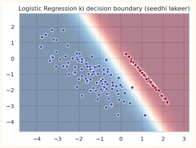
Gehra laal ya neela hissa = model ko class par bohat yaqeen, beech ka safed hissa = 50-50 (boundary). Dhyan do: logistic regression sirf seedhi (linear) boundary bana sakti hai. Pecheeda shakal ke liye doosre algorithms aayenge.
14.4 Multiclass Classification
Do se zyada classes (jaise Iris ki 3 species) ke liye logistic regression softmax istemal karti hai: har class ki probability nikalti hai aur sab ka jama 1 hota hai.
from sklearn.datasets import load_iris
iris = load_iris(as_frame=True)
Xi_train, Xi_test, yi_train, yi_test = train_test_split(iris.data, iris.target,
test_size=0.2,
                                                        random_state=42,
stratify=iris.target)
multi = make_pipeline(StandardScaler(), LogisticRegression(max_iter=1000)).fit(Xi_train,
yi_train)
print("Accuracy:", round(multi.score(Xi_test, yi_test), 3))
print("Ek phool ki probabilities (setosa, versicolor, virginica):")
print(multi.predict_proba(Xi_test.iloc[[0]]).round(3), "-> sab ka jama =",
multi.predict_proba(Xi_test.iloc[[0]]).sum())
OUTPUT
Accuracy: 0.933
Ek phool ki probabilities (setosa, versicolor, virginica):
[[0.979 0.021 0.   ]] -> sab ka jama = 1.0
Regularization: parameter C
Logistic regression me regularization ka parameter C hai, aur ye alpha ka ulta hai: C chhota = zyada saza (saada model) , C bara = kam saza . Default C = 1 hai.
for C in [0.001, 0.01, 1, 100]:
    m = make_pipeline(StandardScaler(), LogisticRegression(C=C, max_iter=2000)).fit(X_train,
y_train)
    print(f"C = {C:>6}: train = {m.score(X_train, y_train):.3f} | test = {m.score(X_test,
y_test):.3f}")
OUTPUT
C =  0.001: train = 0.888 | test = 0.930
C =   0.01: train = 0.956 | test = 0.947
C =      1: train = 0.989 | test = 0.982
C =    100: train = 0.993 | test = 0.947
14.5 Classification ko parakhna: Confusion Matrix
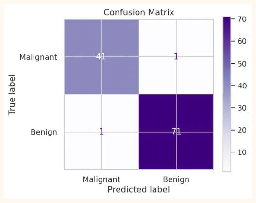
Sirf accuracy kafi nahi. Humein ye bhi jaanna hai ke model kaunsi qism ki ghaltiyan kar raha hai. Iske liye Confusion Matrix hoti hai. Cancer detection ki misaal ( Positive = bimari hai ):
| Model ne kaha: bimari NAHI | Model ne kaha: bimari HAI | |
|---|---|---|
| Asal me bimari NAHI | TN(True Negative): sahi, healthy ko healthy kaha | FP(False Positive): ghalat, healthy ko bimar kaha (jhoota alarm) |
| Asal me bimari HAI | FN(False Negative): ghalat, bimar ko healthy kaha (khatarnak!) | TP(True Positive): sahi, bimar ko bimar kaha |
OUTPUT
[[41  1]
 [ 1 71]]
TP, FP, FN, TN (malignant ko positive maan kar): 41 1 1 71
fig, ax = plt.subplots(figsize=(4.8, 4))
ConfusionMatrixDisplay.from_predictions(y_test, pred, display_labels=["Malignant",
"Benign"],
                                        cmap="Purples", ax=ax)
ax.set_title("Confusion Matrix")
plt.show()
OUTPUT (chart)
14.6 Accuracy, Precision, Recall, F1
| Metric | Formula | Sawal jis ka jawab deta hai |
|---|---|---|
| Accuracy | (TP + TN) / kul | Kul kitne andaze sahi the? |
| Precision | TP / (TP + FP) | Jab model ne "positive" kaha, to kitni bar sahi tha? (jhoote alarm kitne?) |
| Recall(Sensitivity) | TP / (TP + FN) | Jitne asli positive the, un me se kitne pakde? (kitne chhoot gaye?) |
| Specificity | TN / (TN + FP) | Jitne asli negative the, un me se kitne sahi pehchane? |
| F1-score | 2 x P x R / (P + R) | Precision aur Recall ka balanced milap |
OUTPUT
Accuracy : 0.982
Precision: 0.986
Recall   : 0.986
F1       : 0.986
              precision    recall  f1-score   support
   Malignant       0.98      0.98      0.98        42
      Benign       0.99      0.99      0.99        72
    accuracy                           0.98       114
   macro avg       0.98      0.98      0.98       114
weighted avg       0.98      0.98      0.98       114
classification_report har class ke liye precision, recall, f1 aur support (us class ke kitne samples the) ek sath dikha deta hai. Is dataset me Malignant ka recall sab se ahem hai: jitne asli kharab case the, model ne un me se kitne pakde.
Kab kaunsa metric?
| Surat | Kya zyada ahem | Misaal |
|---|---|---|
| FN bohat mehnga | Recall | Cancer detection, fraud pakadna, aag ka alarm |
| FP bohat mehnga | Precision | Spam filter (ahem email ko spam keh dena), kisi begunah par jurm ka ilzam |
| Dono ka balance chahiye | F1-score | Aam classification, imbalanced data |
| Classes barabar hon | Accuracy bhi theek | Barabar classes ka dataset |
14.7 Imbalanced Data aur Accuracy ka dhoka
Fraud detection me 1000 me se sirf 10 transactions fraud hoti hain (1%). Ek model jo hamesha "fraud nahi" kahe, uski accuracy 99% hogi, magar wo ek bhi fraud nahi pakadta . Ye Accuracy Paradox hai.
np.random.seed(0)
y_true = np.array([1] * 10 + [0] * 990)      # 1% fraud
y_lazy = np.zeros(1000, dtype=int)           # hamesha "fraud nahi"
print("Accuracy:", accuracy_score(y_true, y_lazy))
print("Recall  :", recall_score(y_true, y_lazy))        # 0.0: ek bhi nahi pakda
OUTPUT
Accuracy: 0.99
Recall  : 0.0
Imbalanced data ke liye precision, recall, F1, ROC-AUC dekho, aur ye tareeqay aazmao:
-
class_weight="balanced" (chhoti class ko zyada wazan): LogisticRegression(class_weight="balanced") .
-
Oversampling / Undersampling (chhoti class ke nuqtay barhana ya badi class ke kam karna). SMOTE ek mashhoor tareeqa hai.
-
Threshold badalna (neeche dekho).
-
stratify=y ke saath split, aur stratified cross-validation.
14.8 ROC Curve aur AUC
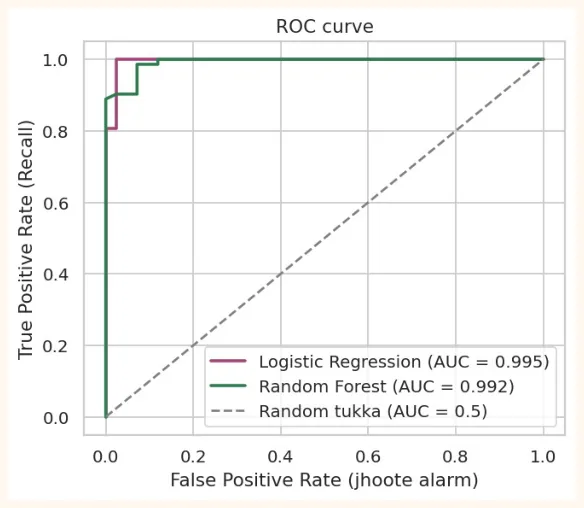
Logistic regression probability deti hai, aur threshold (default 0.5) tay karta hai ke class kya hogi. Threshold badalne se precision aur recall badalte hain. ROC curve ek hi chart me har mumkin threshold par model ka haal dikhati hai:
-
Y-axis: TPR (True Positive Rate = Recall).
-
X-axis: FPR (False Positive Rate = FP / (FP + TN)): jhoote alarm.
-
Behtareen model ka curve upar-left kone ki taraf jata hai. Seedhi tirchi lakeer (diagonal) = andhera tukka (random).
-
AUC (Area Under Curve): curve ke neeche ka rakba. 1.0 = mukammal , 0.5 = random .
from sklearn.metrics import roc_curve, roc_auc_score
from sklearn.ensemble import RandomForestClassifier
proba = clf.predict_proba(X_test)[:, 1]
rf = RandomForestClassifier(random_state=0).fit(X_train, y_train)
proba_rf = rf.predict_proba(X_test)[:, 1]
plt.figure(figsize=(5.6, 4.6))
for name, p, color in [("Logistic Regression", proba, "#A4457A"), ("Random Forest",
proba_rf, "#2F7D4F")]:
    fpr, tpr, _ = roc_curve(y_test, p)
    plt.plot(fpr, tpr, color=color, linewidth=2, label=f"{name} (AUC =
{roc_auc_score(y_test, p):.3f})")
plt.plot([0, 1], [0, 1], linestyle="--", color="gray", label="Random tukka (AUC = 0.5)")
plt.xlabel("False Positive Rate (jhoote alarm)")
plt.ylabel("True Positive Rate (Recall)")
plt.title("ROC curve")
plt.legend(loc="lower right")
plt.show()
OUTPUT (chart)
Threshold tuning: recall ko barhana
Agar cancer detection me recall ahem hai (bimar na chhooten), to hum threshold kam kar sakte hain. Is se model zyada logon ko "shak" me daalta hai: recall barhta hai magar precision girti hai.
p_malignant = clf.predict_proba(X_test)[:, 0]          # malignant (class 0) ki probability
actual_malignant = (y_test == 0).values
for thr in [0.5, 0.2, 0.05, 0.01]:
    flagged = p_malignant >= thr                       # in ko "malignant" kaha
    tp = (flagged & actual_malignant).sum()
    fp = (flagged & ~actual_malignant).sum()
    fn = (~flagged & actual_malignant).sum()
    print(f"threshold {thr}: pakde = {tp}, jhoote alarm = {fp}, chhoot gaye = {fn}")
OUTPUT
threshold 0.5: pakde = 41, jhoote alarm = 1, chhoot gaye = 1
threshold 0.2: pakde = 41, jhoote alarm = 6, chhoot gaye = 1
threshold 0.05: pakde = 42, jhoote alarm = 18, chhoot gaye = 0
threshold 0.01: pakde = 42, jhoote alarm = 30, chhoot gaye = 0
Threshold 0.5 par ek malignant case chhoot gaya (FN = 1). Threshold ko 0.05 tak girane par wo bhi pakda gaya (FN = 0), magar jhoote alarm (FP) 1 se barh kar 18 ho gaye: 18 healthy logon ko bhi "shak" me daal diya gaya. Ye precision aur recall ka sauda hai. Kaunsa threshold chunna hai wo business/medical zaroorat par depend karta hai (cancer me shayad recall zyada ahem, spam filter me precision), na ke sirf data par.
AAM GALTIYAN
-
Sirf accuracy dekhna, khaaskar imbalanced data me.
-
Precision aur Recall ko ulta samajhna. Recall = kitne asli positive pakde , Precision = jo positive kaha unme se kitne sahi .
-
Scaling bhool jana (logistic regression gradient descent aur regularization istemal karti hai).
-
Default threshold (0.5) ko hamesha sahi samajhna.
-
Test set par threshold tune karna. Tuning ke liye validation set ya cross-validation use karo.
-
Regression ke metrics (R<sup>2</sup> , RMSE) classification par lagana.
-
Confusion matrix me rows aur columns ka order ulta parhna (sklearn me rows = asli, columns = andaza).
14.9 Hands-on
-
Baseline: breast cancer par DummyClassifier(strategy="most_frequent") ki accuracy aur recall (malignant ke liye) nikalo.
-
C ka asar: C = 0.01, 0.1, 1, 10 par test accuracy aur ROC-AUC compare karo.
-
class_weight: LogisticRegression(class_weight="balanced") laga kar confusion matrix dekho. Kya recall behtar hua?
-
Threshold: 14.8 wale code me threshold 0.05 aur 0.9 bhi aazmao. Kab FN = 0 ho jata hai aur uski qeemat kya hai?
-
Sochne wala sawal: spam filter ke liye kaunsa metric zyada ahem hoga aur kyun? (FP ya FN kaunsa mehnga hai?)
from sklearn.dummy import DummyClassifier
dummy = DummyClassifier(strategy="most_frequent").fit(X_train, y_train)
print("Baseline accuracy:", round(dummy.score(X_test, y_test), 3))
print("Baseline recall (malignant):", recall_score(y_test, dummy.predict(X_test),
pos_label=0))
balanced = make_pipeline(StandardScaler(), LogisticRegression(class_weight="balanced",
max_iter=1000)).fit(X_train, y_train)
print("Balanced model recall (malignant):", round(recall_score(y_test,
balanced.predict(X_test), pos_label=0), 3))
print("Normal model recall (malignant)  :", round(recall_score(y_test, pred, pos_label=0),
3))
OUTPUT
Baseline accuracy: 0.632
Baseline recall (malignant): 0.0
Balanced model recall (malignant): 0.976
Normal model recall (malignant)  : 0.976
KEY TAKEAWAYS
-
Classification me category ka andaza lagate hain. Logistic Regression ek classification algorithm hai (naam me regression ke bawajood).
-
Sigmoid score ko 0 se 1 ki probability bana deta hai. Threshold (default 0.5) se class tay hoti hai.
-
predict() class deta hai, predict_proba() probability. Coefficients se odds ratio nikalte hain (interpretable model).
-
C regularization ka parameter hai (alpha ka ulta): chhota C = zyada saza.
-
Confusion Matrix: TP, FP, FN, TN. FP = jhoota alarm, FN = chhoot gaya (aksar zyada khatarnak).
-
Precision = jo positive kaha unme se sahi. Recall = asli positives me se pakde. F1 dono ka balance.
-
Imbalanced data me accuracy dhoka hai. ROC-AUC threshold se aazad hai (1 behtareen, 0.5 random). Threshold business zaroorat se chuno.