Chapter 15: Decision Trees aur Random Forests
MODULE 4 | WEEK 15
Chapter 15: Decision Trees aur Random Forests
Ab tak ke models (linear aur logistic regression) ek seedhi lakeer ya formula par chalte the. Decision Tree bilkul alag soch hai: ye data se sawalon ka ek silsila seekhta hai, bilkul insaan ki tarah faisla karne ka tareeqa. Phir Random Forest bohat saray trees ko mila kar ek bohat taqatwar model banata hai. Ye dono algorithms real duniya me sab se zyada istemal hone walon me se hain.
15.1 Decision Tree ka idea
OUTPUT (chart)
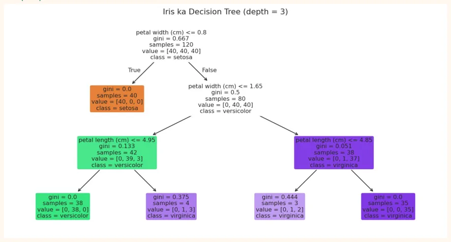
Har dibba batata hai: sawal , gini (impurity, neeche samjhayenge), samples (kitne data points yahan pohanche), value (har class ke kitne samples) aur class (sab se zyada wali). Rang class dikhata hai: jitna gehra, utna "pure" dibba.
Isi tree ko text me bhi dekh sakte hain, jo bilkul if / else rules ki tarah parha jata hai:
print(export_text(tree, feature_names=list(X.columns)))
print("Test accuracy:", round(tree.score(X_test, y_test), 3))
OUTPUT
|--- petal width (cm) <= 0.80
|   |--- class: 0
|--- petal width (cm) >  0.80
|   |--- petal width (cm) <= 1.65
|   |   |--- petal length (cm) <= 4.95
|   |   |   |--- class: 1
|   |   |--- petal length (cm) >  4.95
|   |   |   |--- class: 2
|   |--- petal width (cm) >  1.65
|   |   |--- petal length (cm) <= 4.85
|   |   |   |--- class: 2
|   |   |--- petal length (cm) >  4.85
|   |   |   |--- class: 2
Test accuracy: 0.967
Dekho: tree ne khud rules seekh liye (jaise "agar petal length chhoti hai to setosa"). Isi liye trees samajhne me bohat aasan (interpretable) mane jate hain, aur logon ko mazeed samjhana asaan hota hai.
15.2 Tree sawal kaise chunta hai? Impurity aur Information Gain
Tree har node par wo sawal chunta hai jo data ko sab se saaf (pure) hisson me bant de. "Saaf" napne ke liye impurity ka paimana hota hai:
| Measure | Formula | Range | Matlab |
|---|---|---|---|
| Gini impurity(sklearn ka | 1 - sum(p<sup>2</sup>) | 0 se 0.5 (2 classes) | 0 = bilkul pure (sirf ek class), zyada = |
| default) | mili juli | ||
| Entropy | - sum(p x log2(p)) | 0 se 1 (2 classes) | 0 = pure, 1 = barabar barabar mix |
OUTPUT
p = 0.0: gini = 0.000 | entropy = 0.000
p = 0.1: gini = 0.180 | entropy = 0.469
p = 0.3: gini = 0.420 | entropy = 0.881
p = 0.5: gini = 0.500 | entropy = 1.000
Information Gain = (split se pehle ki impurity) - (split ke baad ke dono hisson ki impurity ka wazni average). Tree har bar wo sawal (feature aur threshold) chunta hai jis se gain sab se zyada ho. Ye ek greedy tareeqa hai: har qadam par abhi ka behtareen sawal, aage ki soch baghair.
# Ek chhota example: 10 students, kya pass hue? Sawal: "parhai >= 5 ghantay?"
before = gini(6 / 10)                               # 6 pass, 4 fail
left = gini(1 / 4)                                  # < 5 ghantay: 4 students me 1 pass
right = gini(5 / 6)                                 # >= 5 ghantay: 6 students me 5 pass
after = (4 / 10) * left + (6 / 10) * right
print("Pehle impurity :", round(before, 3))
print("Baad impurity  :", round(after, 3))
print("Information Gain:", round(before - after, 3))
OUTPUT
Pehle impurity : 0.48
Baad impurity  : 0.317
Information Gain: 0.163
15.3 Overfitting: tree ki sab se bari kamzori
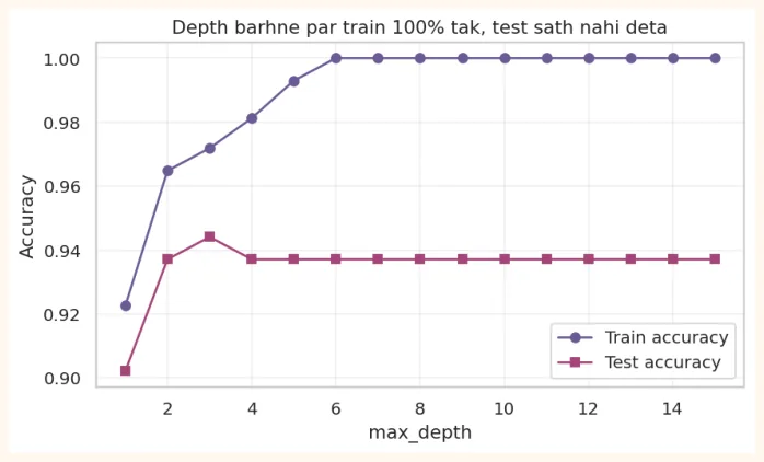
Agar tree ko rokay baghair badhne diya jaye to wo har training sample ko alag leaf me daal kar 100% training accuracy le leta hai, yani data ko ratta maar leta hai (overfitting). Naye data par wo bura chalta hai.
full = DecisionTreeClassifier(random_state=0).fit(X_train, y_train)
print("Poora tree  -> depth:", full.get_depth(), "| leaves:", full.get_n_leaves(),
      "| train:", round(full.score(X_train, y_train), 3), "| test:",
round(full.score(X_test, y_test), 3))
small = DecisionTreeClassifier(max_depth=3, random_state=0).fit(X_train, y_train)
print("Depth = 3   -> depth:", small.get_depth(), "| leaves:", small.get_n_leaves(),
      "| train:", round(small.score(X_train, y_train), 3), "| test:",
round(small.score(X_test, y_test), 3))
OUTPUT
Poora tree  -> depth: 5 | leaves: 8 | train: 1.0 | test: 0.967
Depth = 3   -> depth: 3 | leaves: 5 | train: 0.983 | test: 0.967
Isse bachne ke liye tree ko rokte hain (pruning ki tarah). Ahem hyperparameters:
| Hyperparameter | Kya karta hai |
|---|---|
| max_depth | Tree ki zyada se zyada gehrai |
| min_samples_split | Kisi node ko todne ke liye kam az kam kitne samples chahiye |
| min_samples_leaf | Har leaf me kam az kam kitne samples hon |
| max_leaf_nodes | Zyada se zyada leaves |
| max_features | Har split par kitne features me se chunna hai |
| criterion | "gini" ya "entropy" |
Dekho max_depth badalne par train aur test score ka kya hota hai (breast cancer data par):
from sklearn.datasets import load_breast_cancer
bc = load_breast_cancer(as_frame=True)
Xb_train, Xb_test, yb_train, yb_test = train_test_split(bc.data, bc.target, test_size=0.25,
                                                        random_state=1, stratify=bc.target)
depths = range(1, 16)
train_sc, test_sc = [], []
for d in depths:
    t = DecisionTreeClassifier(max_depth=d, random_state=0).fit(Xb_train, yb_train)
    train_sc.append(t.score(Xb_train, yb_train))
    test_sc.append(t.score(Xb_test, yb_test))
print("Behtareen test accuracy depth:", list(depths)[int(np.argmax(test_sc))], "| score:",
round(max(test_sc), 3))
OUTPUT
Behtareen test accuracy depth: 3 | score: 0.944
plt.figure(figsize=(7.5, 4))
plt.plot(depths, train_sc, marker="o", color="#6B5B95", label="Train accuracy")
plt.plot(depths, test_sc, marker="s", color="#A4457A", label="Test accuracy")
plt.xlabel("max_depth")
plt.ylabel("Accuracy")
plt.title("Depth barhne par train 100% tak, test sath nahi deta")
plt.legend()
plt.grid(alpha=0.3)
plt.show()
OUTPUT (chart)
Decision boundary: tree dibbon me soch'ta hai
Do features par tree ka faisla chaukor hisson (axis-parallel rectangles) me bat'ta hai, kyunke har sawal ek feature par ek threshold hota hai:
from sklearn.inspection import DecisionBoundaryDisplay
from sklearn.datasets import make_moons
Xm, ym = make_moons(n_samples=300, noise=0.3, random_state=0)
fig, axes = plt.subplots(1, 2, figsize=(10, 4))
for ax, depth, title in zip(axes, [3, None], ["max_depth = 3 (saada)", "Koi limit nahi
(overfit)"]):
    m = DecisionTreeClassifier(max_depth=depth, random_state=0).fit(Xm, ym)
    DecisionBoundaryDisplay.from_estimator(m, Xm, ax=ax, alpha=0.4, cmap="coolwarm",
response_method="predict")
    ax.scatter(Xm[:, 0], Xm[:, 1], c=ym, cmap="coolwarm", edgecolor="white", s=22)
    ax.set_title(title)
plt.tight_layout()
plt.show()
OUTPUT (chart)
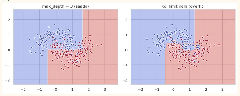
Doosre chart me boundary bohat ghumavdar aur choti choti jazeeron me bat gayi hai: tree ne har ek noise wale nuqtay ko bhi alag class me daal diya. Ye overfitting ki tasveer hai.
15.4 Decision Tree Regression
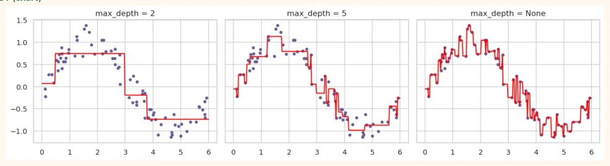
Trees sirf classes nahi, numbers ka bhi andaza lagate hain. Leaf me us hisse ke samples ka average hota hai. Is ka nateeja seedhi lakeer nahi, seedhiyon (steps) ki shakal hota hai.
from sklearn.tree import DecisionTreeRegressor
np.random.seed(0)
xr = np.sort(np.random.uniform(0, 6, 80)).reshape(-1, 1)
yr = np.sin(xr).ravel() + np.random.normal(0, 0.2, 80)
xs = np.linspace(0, 6, 300).reshape(-1, 1)
fig, axes = plt.subplots(1, 3, figsize=(13, 3.5), sharey=True)
for ax, d in zip(axes, [2, 5, None]):
    m = DecisionTreeRegressor(max_depth=d, random_state=0).fit(xr, yr)
    ax.scatter(xr, yr, color="#6B5B95", s=14)
    ax.plot(xs, m.predict(xs), color="red")
    ax.set_title(f"max_depth = {d}")
plt.tight_layout()
plt.show()
OUTPUT (chart)
15.5 Feature Importance
Tree batata hai ke kaunsa feature faislon me sab se zyada kaam aaya. Har feature ki importance uske lagaye hue splits se kitni impurity kam hui us se napi jati hai (sab ka jama 1 hota hai).
t = DecisionTreeClassifier(max_depth=4, random_state=0).fit(Xb_train, yb_train)
imp = pd.Series(t.feature_importances_, index=bc.data.columns).sort_values(ascending=False)
print(imp.head(5).round(3))
OUTPUT
worst concave points    0.751
worst area              0.138
mean texture            0.031
worst radius            0.030
worst texture           0.019
dtype: float64
AAM GALTIYAN
-
Feature importance ko wajah samajhna. Ye sirf batati hai ke model ne kis ko zyada istemal kiya, na ke asli duniya me kaun wajah hai.
-
Importance ka correlated features me bant jana: do milte julte features ki importance aadhi aadhi ho sakti hai, ya ek ko saari mil jati hai.
-
Tree ko bina limit ke chhor dena (overfit).
-
Data me bohat categories wale columns (jaise 500 shehar) par seedha tree lagana.
15.6 Ensemble Learning aur Random Forest
Ek akela tree kamzor aur be-bharosa hota hai: data me thori si tabdeeli par bilkul alag tree ban jata hai (isay high variance kehte hain). Ensemble Learning ka idea: bohat saray kamzor models mila kar ek mazboot model banao .
Bagging (Bootstrap Aggregating)
-
Training data se bar bar random sample lo, wapas rakh kar (bootstrap): har sample me kuch rows 2-3 bar aati hain aur kuch ayi hi nahi.
-
Har sample par ek alag tree train karo.
-
Naye data par sab trees se vote (classification) ya average (regression) lo.
Random Forest = Bagging + Random Features
Random Forest bagging ke saath ek aur chalaki karta hai: har tree ke har split par sirf features ka ek random hissa ( max_features ) dekhne ki ijazat hoti hai. Is se saray trees ek jaise nahi bante ( decorrelated ), aur ensemble zyada mazboot hota hai.
| Cheez | Kya hota hai |
|---|---|
| n_estimators | Kitne trees (zyada = behtar aur stable, magar slow). Aam taur par 100 se 500 |
| max_features | Har split par kitne features dekhne hain (classification me aam taur par sqrt(kul features)) |
| max_depth, min_samples_leaf | Har tree ka size (wohi hyperparameters jo upar dekhe) |
| bootstrap=True | Har tree alag random sample par train hota hai |
| oob_score=True | Out-of-Bag score: wo rows jo kisi tree ke sample me aayi hi nahi, un par free validation |
| n_jobs=-1 | Saray CPU cores istemal karo (tez) |
| random_state | Nateeja dobara dohraya ja sake |
from sklearn.ensemble import RandomForestClassifier
tree1 = DecisionTreeClassifier(random_state=0).fit(Xb_train, yb_train)
rf = RandomForestClassifier(n_estimators=200, oob_score=True, random_state=0, n_jobs=-
1).fit(Xb_train, yb_train)
print("Akela Decision Tree test accuracy:", round(tree1.score(Xb_test, yb_test), 3))
print("Random Forest test accuracy       :", round(rf.score(Xb_test, yb_test), 3))
print("Random Forest OOB score           :", round(rf.oob_score_, 3))
OUTPUT
Akela Decision Tree test accuracy: 0.937
Random Forest test accuracy       : 0.944
Random Forest OOB score           : 0.962
OOB score ek muft ka validation hai: har tree ne apni training me data ka ~37% kabhi dekha hi nahi, isliye us par tree ki parakh hoti hai. Alag validation set banane ki zaroorat nahi.
Trees ki tadaad barhane ka asar
for n in [1, 5, 20, 100, 400]:
    m = RandomForestClassifier(n_estimators=n, random_state=0, n_jobs=-1).fit(Xb_train,
yb_train)
print(f"n_estimators = {n:>3}: test accuracy = {m.score(Xb_test, yb_test):.3f}")
OUTPUT
n_estimators =   1: test accuracy = 0.895
n_estimators =   5: test accuracy = 0.944
n_estimators =  20: test accuracy = 0.951
n_estimators = 100: test accuracy = 0.944
n_estimators = 400: test accuracy = 0.944
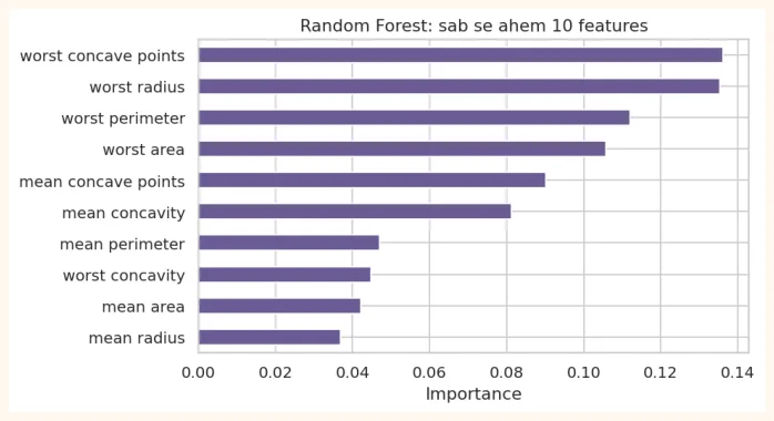
Random Forest ki feature importance
imp = pd.Series(rf.feature_importances_, index=bc.data.columns).sort_values().tail(10)
plt.figure(figsize=(7, 4))
imp.plot(kind="barh", color="#6B5B95")
plt.title("Random Forest: sab se ahem 10 features")
plt.xlabel("Importance")
plt.show()
OUTPUT (chart)
Random Forest regression
from sklearn.ensemble import RandomForestRegressor
from sklearn.datasets import load_diabetes
from sklearn.linear_model import LinearRegression
dX, dy = load_diabetes(return_X_y=True)
dXtr, dXte, dytr, dyte = train_test_split(dX, dy, test_size=0.2, random_state=42)
for name, m in [("Linear Regression", LinearRegression()),
                ("Decision Tree", DecisionTreeRegressor(random_state=0)),
                ("Random Forest", RandomForestRegressor(n_estimators=200, random_state=0,
n_jobs=-1))]:
    m.fit(dXtr, dytr)
    print(f"{name:18s} test R2 = {m.score(dXte, dyte):.3f}")
OUTPUT
Linear Regression  test R2 = 0.453
Decision Tree      test R2 = -0.003
Random Forest      test R2 = 0.420
Dhyan do: akela Decision Tree ka R<sup>2</sup> lagbhag 0 hai (poori tarah overfit), Random Forest us se kaafi behtar hai, magar is chhote aur shor wale dataset par seedhi linear regression abhi bhi barabar ya behtar hai. Sabaq: har data par pecheeda model behtar nahi hota , hamesha saade model se muqabla karo.
15.7 Boosting ka taruf
Bagging me trees ek sath (parallel) aur aapas me alag alag banti hain. Boosting me trees ek ke baad ek (sequence) banti hain, aur har nayi tree pichli trees ki ghaltiyan theek karne par focus karti hai .
OUTPUT
Gradient Boosting         : 0.958
HistGradientBoosting (tez): 0.958
Table data (rows aur columns wala data) par Gradient Boosting aur uski mashhoor libraries ( XGBoost, LightGBM, CatBoost ) aksar sab se behtareen nateeje deti hain aur Kaggle competitions me bohat mashhoor hain. Hum yahan sirf pehchan tak rahenge.
15.8 Trees ke fayde aur nuqsan
| Decision Tree / Random Forest ke fayde | Nuqsan |
|---|---|
| Scaling ki zarooratnahi | Single tree jaldi overfit hota hai |
| Numeric aur categorical dono ke saath kaam | Random Forest ko samajhna mushkil (black box jaisa) |
| Non-linearrishton aur feature interactions ko khud seekhta hai | Bari forest memory aur waqt leti hai |
| Outliers se kam mutasir | Data ki range se bahar andaza nahi (regression) |
| Single treesamajhne me aasan | Bohat zyada categories wale features me masla |
| Feature importance milti hai | Seedhe linear rishton me linear models se kam efficient |
15.9 Hands-on
Seaborn ke titanic dataset par (kaun bacha?) ek chhota workflow:
import seaborn as sns
titanic = sns.load_dataset("titanic")
df = titanic[["survived", "pclass", "sex", "age", "sibsp", "parch", "fare"]].copy()
print(df.shape, "| missing age:", df["age"].isnull().sum())
print(df["survived"].value_counts(normalize=True).round(3).to_dict())
OUTPUT
(891, 7) | missing age: 177
{0: 0.616, 1: 0.384}
df["age"] = df["age"].fillna(df["age"].median())
df["sex"] = (df["sex"] == "female").astype(int)           # female = 1
Xt, yt = df.drop(columns="survived"), df["survived"]
Xt_tr, Xt_te, yt_tr, yt_te = train_test_split(Xt, yt, test_size=0.2, random_state=42,
stratify=yt)
print("Baseline (sab ko 'mar gaya' kaho):", round(1 - yt_te.mean(), 3))
for name, m in [("Decision Tree (depth 4)", DecisionTreeClassifier(max_depth=4,
random_state=0)),
                ("Random Forest", RandomForestClassifier(n_estimators=300,
min_samples_leaf=3, random_state=0, n_jobs=-1))]:
    m.fit(Xt_tr, yt_tr)
    print(f"{name:24s} test accuracy = {m.score(Xt_te, yt_te):.3f}")
rf_t = RandomForestClassifier(n_estimators=300, min_samples_leaf=3, random_state=0, n_jobs=-
1).fit(Xt_tr, yt_tr)
print(pd.Series(rf_t.feature_importances_,
index=Xt.columns).sort_values(ascending=False).round(3))
OUTPUT
Baseline (sab ko 'mar gaya' kaho): 0.615
Decision Tree (depth 4)  test accuracy = 0.777
Random Forest            test accuracy = 0.793
sex       0.382
fare      0.246
age       0.176
pclass    0.117
sibsp     0.044
parch     0.035
dtype: float64
-
Tree dekho: Titanic ka depth = 3 tree plot_tree se banao. Root par kaunsa sawal hai?
-
Depth curve: max_depth 1 se 12 tak train aur test accuracy plot karo.
-
min_samples_leaf: 1, 5, 20 par test score compare karo.
-
Forest: n_estimators ko 10, 100, 500 karke OOB score dekho.
-
Sochne wala sawal: feature importance me sex upar kyun hai? Is ka matlab ye hai ke jins wajah thi, ya sirf ek nishani?
KEY TAKEAWAYS
-
Decision Tree data se sawalon ka silsila seekhta hai (if / else rules). Samajhne me aasan, scaling ki zaroorat nahi.
-
Split ka mayar: Gini ya Entropy impurity, jo Information Gain sab se zyada ho wo sawal chuna jata hai.
-
Bina limit ke tree overfit hota hai. max_depth, min_samples_leaf waghera se roko.
-
Ensemble: bohat saray kamzor models ka milap. Bagging parallel (bootstrap), Boosting ek ke baad ek (ghaltiyan theek karte hue).
-
Random Forest = bagging + har split par random features. Akele tree se kaafi behtar aur stable. OOB score muft validation hai.
-
n_estimators barhane se aam taur par nateeja behtar ya stable hota hai. max_features, max_depth, min_samples_leaf se control.
-
Feature importance batati hai model ne kis ka zyada istemal kiya, wajah nahi. Table data par Gradient Boosting aksar sab se behtareen hota hai.